Musings: January - April 2018 (archive)

Home > Musings: Main > Archive > Archive for January-April 2018 (this page) | Introduction | e-mail announcements | Contact

Musings: January - April 2018 (archive)

Musings is an informal newsletter mainly highlighting recent science. It is intended as both fun and instructive. Items are posted a few times each week. See the Introduction, listed below, for more information.

If you got here from a search engine... Do a simple text search of this page to find your topic. Searches for a single word (or root) are most likely to work.

If you would like to get an e-mail announcement of the new posts each week, you can sign up at e-mail announcements.

Introduction (separate page).
This page:
2018 (January-April)
April 30 April 25 April 18 April 11 April 4 March 28 March 21 March 14 March 7 February 28 February 21 February 14 February 7 January 31 January 24 January 17 January 10 January 3

Also see the complete listing of Musings pages, immediately below.

Links to external sites will open in a new window.

Archive items may be edited, to condense them a bit or to update links. Some links may require a subscription for full access, but I try to provide at least one useful open source for most items.

Please let me know of any broken links you find -- on my Musings pages or any of my web pages. Personal reports are often the first way I find out about such a problem.

April 30, 2018

Sudden infant death: a genetic factor affecting breathing?

April 30, 2018

Sometimes a baby goes to sleep -- and dies. It's called sudden infant death syndrome (SIDS), or, casually, crib death. In places with generally low levels of infant infection, it may be the leading cause of infant death.

There is no warning, and little explanation. It is probably respiratory failure, but why? Efforts to make sure babies sleep on their backs, and are not buried under things that might obstruct breathing, have led to a decrease in the rate of SIDS, but the condition is still largely mysterious.

A new article uncovers a genetic condition that may contribute to SIDS for some babies. It's an interesting clue, and it may even lead to a treatment. It is also a very small piece of the story.

The scientists did genome sequencing for a group of babies who had died of SIDS, and a group of healthy controls. They focused on regions suspected of having relevant genes. The results for one particular gene stood out. 1.4% of the babies who died of SIDS carried a mutation that altered the function of a particular gene, called SCN4A. None of the controls carried such mutations. We'll skip the detail of the numbers here, but that difference tested as significant. Further, the relevant mutations are all considered extremely rare as judged by genome databases.

What is this gene? A gene for a particular type of ion channel, which controls skeletal respiratory muscle function.

Previous work had shown that some babies who die of SIDS have an ion channel mutation that affects heart rhythm.

The following figure shows an example of the effect of one of the mutations, based on work in a lab model.

The test here measures the ion channels in lab cells that have been modified to have the mutant gene of interest. The graphs show the electrical current as a function of time. Time is a stand-in here for voltage. The voltage is increased over time, and the resulting current is measured.

The left frame is for the wild type ion channel. The right frame is for one of the mutant ion channels found in a baby who had died from SIDS. It's clear that the mutant channel is different. The spike in current at about 1 ms represents the activation of the channel. The mutant channel doesn't activate well.

The details vary for each mutant channel studied. What is common is that for each case that was finally counted as contributing there was a distinct change in ion channel performance.

This is Figure 2A from the article.

Overall... A small number of babies who died from SIDS have a mutation that affects their breathing muscles. Suspicious, isn't it? But remember that such mutations are found in only 1.4% of the cases, and no causal link has been established. It may be a clue, but it is only that for now.

As an example of what might be happening... It may be that the mutation weakens the breathing system, making the baby more vulnerable to a stress.

There are drugs that can modulate such ion channels. Might they be useful in preventing SIDS? Again, it can only be a lead for now -- but leads are a good place to start.

News stories:
* Rare Gene Variant Tied to SIDS -- Genes controlling breathing muscle function could be important. (M Walker, MedPage Today, March 29, 2018.)
* Potential genetic link in sudden infant death syndrome identified. (Science Daily, March 28, 2018.)

Both of the following are freely available.
* "Comment" accompanying the article: Skeletal muscle channelopathy: a new risk for sudden infant death syndrome. (S C Cannon, Lancet 391:1457, April 14, 2018.)
* The article: Dysfunction of NaV1.4, a skeletal muscle voltage-gated sodium channel, in sudden infant death syndrome: a case-control study. (R Männikkö et al, Lancet 391:1483, April 14, 2018.)

Previous posts on SIDS: none.

More SIDS: A bio-marker for SIDS? (June 27, 2022).

A post that notes the issue of child mortality: Ten Great Public Health Achievements, 2001-2010 (June 26, 2011).

Previous post on voltage-gated sodium channels: A long worm with a novel toxin (April 28, 2018). Immediately below.

A long worm with a novel toxin

April 28, 2018

Imagine you are walking by a building, and a worm crawls out of a window on the third floor. It reaches down and bites you -- while still holding on to its third-floor perch.

Now imagine a similar scenario, but the worm is on the 15th floor.

We have a new article about the toxin produced by a worm, but it's the worm that is getting the attention. The special feature of the worm is noted in the title of the article, and in the title of all the news stories I saw.

The worm is the bootlace worm, Lineus longissimus. It's a type of ribbon worm, a group that has not been studied much. It's very long. In fact, it is the longest known animal. The longest specimen known is about 55 meters (about 180 feet). That's nearly twice the length of the longest known whale. It's long enough to get you from the 15th floor. It's about a centimeter wide -- ribbon-like, indeed.

The report of a 55 m worm goes back over a century. I don't know how reliable it is. More typical are worms 10 m or so. Long enough to get you from the 3rd floor.

These are marine worms. They don't live in tall buildings. And they don't attack humans. I think. The opening of this post was to establish a sense of scale, not their ecology.

The toxin? This worm makes a toxin that can kill medium size arthropods, such as crabs. In the current work, the scientists isolated the toxin, determined its structure, and explored its function. They also looked for related toxins from other worms of the group.

Here are the worm and the toxin. They are shown here at about the same size.


The worm	The toxin
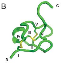
The worm is from the Phys.org news story. There is no scale given. We might guess that it is about a centimeter wide, and a few meters long. The toxin is from Figure 4B of the article. It's a protein -- actually a 31-amino acid peptide. It's shown here as a computer-generated ribbon, one common way to show protein structures. This small peptide is probably about a nanometer across. In the toxin structure, N and C mark the amino and carboxyl termini. The Roman numerals are for cysteine residues that pair off to form disulfide bonds (which are themselves yellow). The article does have a picture of the animal (Figure 1A), but it's partly folded up. (One of the news stories has a picture of the worm completely folded up into a ball.)

Is this toxin of interest? Maybe. The scientists show that it is very effective against ion channels in the nervous system of arthropods. It has much less effect on mammalian ion channels. Thus it -- and related peptide toxins found in related worms -- might be considered as the basis for development of novel insecticides. Perhaps this is worth exploring further. At some point, it might be possible to talk about the toxin without noting that it is from the world's longest animal.

News stories:
* Bootlace Worm: Earth's Longest Animal Produces Powerful Toxin. (Sci.news, March 27, 2018.)
* TIL: The World's Longest Animal Is Over 50 Meters Long and It's A Worm! ("trumpman", steemit, March 23, 2018.) A blog post on a site I had not seen before. Useful story, with a couple of worm videos.
* Potential insecticide discovered in Earth's longest animal. (Phys.org, March 23, 2018.)

The article, which is freely available: Peptide ion channel toxins from the bootlace worm, the longest animal on Earth. (E Jacobsson et al, Scientific Reports, 8:4596, March 22, 2018.) It's a very readable article, with some discussion of the worms, and considerable discussion of neurotoxins from a wide range of sources.

Previous post featuring the longest of something: The longest C-C bond (April 17, 2018).

Previous post about a worm: Why you should not eat larb: A story of trichinellosis -- locally (March 11, 2018).

More on novel insecticides:
* A case of horizontal gene transfer from plant to insect; exploiting it for insect control (April 18, 2021).
* Alternative microbial sources of insecticidal proteins (December 9, 2016).

Next post on voltage-gated sodium channels: Sudden infant death: a genetic factor affecting breathing? (April 30, 2018). Immediately above.

Ancient DNA and the archeologists

April 27, 2018

Archaeology -- a study of ancient humans -- has a new tool. Genome sequencing is one of the revolutionary developments of recent years. A symbol, or reference point, for this revolution was the announcement of the first complete human genome sequence in 2001. Ancient DNA presents special challenges, but these have been addressed. Since 2010 scientists have sequenced the genomes of 1300 ancient humans. Half of those are from the current year -- which is still very much in progress.

A new tool and a lot of data. Not all the new data agrees with what the archeologists thought they knew.

A recent News Feature from Nature explores the role of sequencing ancient genomes in modern archeology. It's not a simple story, but it is a good story about how science progresses. Worth a browse.

News feature. which is freely available: Divided by DNA: The uneasy relationship between archaeology and ancient genomics -- Two fields in the midst of a technological revolution are struggling to reconcile their views of the past. (E Callaway, Nature News, March 28, 2018.) In print, with the title The Battle for Common Ground... Nature 555:573 (March 29, 2018).

The article has a graphic showing the number of ancient human genomes reported per year.

* * * * *

A post about the very first ancient human genome that was published: Inuk, a 4000 year old Saqqaq from Qeqertasussuk (March 1, 2010).

There is more about DNA sequencing on my page Biotechnology in the News (BITN) - DNA and the genome. It includes an extensive list of related Musings posts.

April 25, 2018

Follow-up: bacterial degradation of PET plastic

April 25, 2018

Two years ago Musings reported the isolation of a bacterial strain that could digest one type of polyester plastic, poly(ethylene terephthalate) (PET) [link at the end]. We now have a new article reporting work on the PET-degrading enzyme system from that bacterium. Among other things, the scientists report an improvement in the activity of the main enzyme. The article has been hyped in some of the news reports, but still is of interest.

The following figure introduces the PET polymer, and shows what the bacterial enzymes do to it.

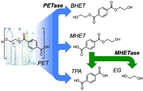
The left side shows the chemical structure of the PET polymer. It is an alternating polymer of terephthalic acid (TPA) and ethylene glycol (EG). If it is new to you, you might start at the lower right, which shows those two monomers.

The right side shows what the enzymes do to PET. Not surprisingly, the enzymes break the ester link between monomers, leading to various smaller molecules. For example, the PETase -- the enzyme that directly attacks the PET-- makes the top two molecules on the right. They consist of TPA with one or two EG attached. Those are called MHET and BHET [mono- and bis-(2-hydroxyethyl)-terephthalic acid], respectively. (MHET is the major product from the PETase enzyme.)

The second enzyme is MHETase. It breaks down MHET to the two original monomers. This is the step at the lower right.

It's of interest that the enzyme system yields the two monomers used to make the plastic. If this process can be made practical, it clearly makes useful products.

This is Figure 1 from the article.

In the new work, the scientists did various biochemical and structural studies on the two enzymes. Along the way, they made a few mutant enzymes, by changing certain amino acids that they thought might be in interesting positions. Of particular interest is one double-mutant enzyme, called W159H,S238F.

As we have noted occasionally, such a name describes the amino acid changes. For example, "W159H" means that amino acid W (tryptophan) at position 159 has been changed to an H (histidine).

The following figure shows some data for the enzymes...

The figure shows some results for how the PETase attacks PET.

There are three sets of data. The middle set is for the wild-type PETase enzyme. The set at the right is for the double mutant enzyme noted above. At the left is a buffer control, with no enzyme.

For each data set, there are three measures of enzyme activity. From the left... loss of crystallinity (green bar), and production of two products: MHET (blue-striped bar) and TPA (black-hatched bar) For crystallinity, use the y-axis scale at the left; for the products, use the scale at the right.

Look first at the results for crystallinity. There is a small loss of crystallinity even in the buffer, but it is enhanced by the enzyme. Further, the mutant enzyme leads to much more loss of crystallinity. (The plastic used here is about 15% crystalline. Thus the highest green bar shows loss of about 1/3 of the original crystallinity.)

Now look at the production of the two small-molecule products. There is none with the buffer control, but significant amounts with the enzymes. There is little difference between the two enzymes here.

This is Figure 3D from the article.

From those results, it seems likely that the enzyme makes random nicks in the polymer structure. That leads to a relatively fast loss of polymer integrity, as reflected in the crystallinity. That the mutant enzyme does this better is encouraging.

By this model, appearance of small products requires two nicks close to each other. That takes more time. Clearly, the enzyme leads to the small-molecule products, but the enzyme improvement isn't reflected by this measure. Note that we have only one time point (96 hours); it would be interesting to see more kinetics.

Overall, the article provides evidence for an improved enzyme. Some of the news coverage has suggested that the article provides a process for degrading PET. However, it is not yet good enough for a practical process. The authors recognize that.

A little more from the article... The authors test the enzyme on other polyester plastics. It does act on another plastic that has an aromatic ring in the monomers, a plastic that may be coming along as a replacement for PET. However, the enzyme does not act on polyesters that lack an aromatic ring.

It's time to repeat the big caution about plastics... There are diverse types of plastic -- as your local recycler will undoubtedly remind you. The work here is on one specific type. It is indeed a major plastic. If this work leads to a practical process for the degradation of PET, that could be important. But there is nothing here that is general for plastics.

News stories:
* Scientists accidentally create mutant enzyme that eats plastic bottles. (D Carrington, Guardian, April 16, 2018.)
* Research Team Engineers a Better Plastic-Degrading Enzyme. (National Renewable Energy Laboratory (NREL), April 16, 2018.) From one of the participating institutions.
* Expert reaction to enzyme to digest plastic. (Science Media Centre, April 16, 2018.) Several comments.

The article, which is freely available: Characterization and engineering of a plastic-degrading aromatic polyesterase. (H P Austin et al, PNAS 115:E4350, May 8, 2018.)

Background post reporting the PET-degrading bacterial strain: Discovery of bacteria that degrade PET plastic (April 3, 2016).

More about getting rid of plastics:
* Good enzymatic degradation of polyesters, by manufacturing the plastic with the enzymes in it (May 4, 2021).
* Turning waste plastic into fuel -- a solar-driven process? (October 9, 2018).

A recent post on plastics: A "greener" way to make acrylonitrile? (January 6, 2018).

This post is listed on my page Internet Resources for Organic and Biochemistry in the section for Carboxylic acids, etc.

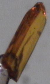
Ice in your diamond?

April 23, 2018

Briefly noted...

A recent article reports evidence for finding ice inside some diamonds.

It's not ordinary ice, but rather an unusual crystal form called ice-VII. As with other inclusions found in diamonds, the ice must have gotten there when the diamond was formed -- deep down inside the Earth. More precisely, the water that formed the ice was included in the diamond upon its formation. That is, the presence of the ice in the diamond is evidence for the presence of liquid water at the site of diamond formation.

Then what? As the diamond -- and its water -- cooled, ice formed. Ice-VII only forms at extremely high pressures -- found only at depths of several hundred kilometers below the surface.

There was a recent report of finding ice-VI in diamonds. The current article is the first report of ice-VII, indicative of even higher pressures, in diamonds.

The conclusion is clear: these diamonds must have formed at great depths. And there must be water -- and aqueous chemistry -- down there. That's useful information; understanding water in Earth's mantle is important, but limited. And finding ice-VII in nature is also new; previously, ice-VII was known only from lab work.

From the title of the post, you may have expected some pictures. Sorry, no pictures. The article contains X-ray pictures to determine the nature of the inclusions, and diagrams of the pressure inside the Earth. These diamonds have a story to tell about Earth's interior, but apparently aren't anything special to look at.

News stories:
* Small Inclusions of Unique Ice in Diamonds Indicate Water Deep in Earth's Mantle. (Sci.news, March 12, 2018.)
* Scientists Just Discovered a Strange New Type of Ice Inside Deep-Earth Diamonds -- We've never seen ice-VII in nature before. (M McRae, Science Alert, March 9, 2018.)
* Diamond inclusions suggest free flowing water at boundary between upper and lower mantle. (B Yirka, Phys.org, March 9, 2018.)

The article: Ice-VII inclusions in diamonds: Evidence for aqueous fluid in Earth's deep mantle. (O Tschauner et al, Science 359:1136, March 9, 2018.)

Previous post about diamonds: The smallest radio receiver (April 4, 2017).

More diamonds: Another Solar System planet -- revealed by its diamonds? (May 22, 2018).

A recent post about ice: Should we geoengineer glaciers to reduce their melting? (April 4, 2018).

More ice:
* Added May 23, 2023. A new ice, with the density of liquid water (May 23, 2023).
* Why is ice slippery? (September 9, 2018).

Fracking and earthquakes: It's injection near the basement that matters

April 22, 2018

Fracking is associated with earthquakes in some places. Quake activity is usually most closely associated with the follow-up process of wastewater injection, but there may also be effects from the fracking injection itself. Background posts discuss both of these possibilities [links at the end].

The work on wastewater disposal has suggested that injection near rigid basement structures that are prone to seismic activity may be of particular concern. A new article reinforces the point.

The article is based on statistical analysis of data from the Oklahoma oil and gas fields. We note one summary figure...

The graph analyzes a large number of wastewater injection sites. Each site is classified by the seismic activity that has been observed there. This is recorded as the total annual seismic moment, in Newton-meters (Nm). In particular, two sub-groups of the sites are featured; those with high seismic activity (pink) and those with low seismic activity (blue). Further, each site is at a known depth, and a known distance from the basement structure at that region.

The y-axis scale is a measure of the probability of such seismic activity. It is plotted against depth of the site in frame A, and against distance from the basement in frame B.

Look first at frame B (bottom). You can see that the pink distribution, for the sites with high seismic activity, clusters very near zero. In contrast, the blue distribution, for sites with low seismic activity, is bimodal, and tends to be away from zero. Remember, in this frame, zero means near the basement.

In contrast, frame A (top) plots the results vs actual depth (rather than depth relative to the basement). Interestingly, the low-seismic sites (blue) are at lower depth.

This is part of Figure 3 from the article.

Overall, the work supports the notion that injection of wastewater near the basement is of special concern. The contribution of the new article is to separate the more specific measure of "distance from basement" from the more general "depth".

Volume injected is also an issue. It becomes increasingly important when injection is near the basement

The authors note that state regulators have implemented some regulations restricting wastewater injections, based on earlier findings. Preliminary data suggests that there is now reduced seismic activity in the area, though there is too little data to be conclusive. The authors hope that their new findings will lead to improved regulations.

The story of fracking and seismic activity has been developing over several years. At first, there were anecdotal reports, with considerable skepticism. There is now general acceptance that there is a problem in certain locations. A stream of scientific studies, such as the current work, has led to some understanding of what is going on; that guides implementation of solutions. At least some regulatory agencies are now actively dealing with the issue. Of course, our current understanding is undoubtedly incomplete, and the analysis must continue.

News stories:
* Wastewater well depths linked to Oklahoma quakes. (E D O'Reilly, Axios, February 1, 2018.)
* Oklahoma's Earthquakes Strongly Linked to Wastewater Injection Depth. (Phys.org, February 1, 2018.)

The article: Oklahoma's induced seismicity strongly linked to wastewater injection depth. (T Hincks et al, Science 359:1251, March 16, 2018.)

Background posts on fracking and earthquakes include:
* Hydraulic fracturing (fracking) and earthquakes: a direct connection (February 13, 2017).
* Fracking: the earthquake connection (June 19, 2015). This is about quakes associated with wastewater disposal.

More about earthquakes...
* Earthquakes induced by human activity: oil drilling in Los Angeles (February 12, 2019).
* A significant local earthquake: identifying a contributing "cause"? (July 31, 2018).
* Detecting earthquakes using the optical fiber cabling that is already installed underground (February 28, 2018).

More fracking: Fracking by mice (November 18, 2019).

More seismic waves... How seismic waves travel through the Earth: effect of redox state (June 8, 2018).

There is more about energy issues on my page Internet Resources for Organic and Biochemistry under Energy resources. It includes a list of some related Musings posts.

Do naked mole rats get old?

April 20, 2018

Aging is not simply about time. A 40-year-old person may be in the prime of life. An 80-year-old is near the end. "The end". The term implies that there is some kind of limit -- a maximum lifespan. Aging is a physiological process near the end of that lifespan.

The following figure illustrates the idea, in a different -- but intriguing -- way.

Simplifying a bit, the figure shows the "mortality hazard" (risk of death) vs "age" for four mammals.

The purple curve near the left is for humans. The mortality hazard is low at the start, then increases dramatically.

The curve for horses is very similar.

The curve for mice is similar, too, but the increase occurs at a later age (on this scale, which we will explain below).

And then there is the green curve. It is for naked mole rats. It, too, starts low -- but this curve stays low.

This is Figure 5E from the article.

In summary, the graph shows that the death rate for three mammals rises dramatically at some point during their life. That is typical of what is found for mammals. However, according to this graph, the naked mole rat doesn't do that. It doesn't age.

Let's look at the graph scales. The y-axis is somewhat arbitrary; there are real numbers, but they are different for the different animals. What matters for the y-axis is the trend. (The numbers are seen more cleanly in the other parts of the full figure, which show the data underlying the graph above on a more conventional scale, vs simple age.)

The x-axis scale is more interesting. Note the vertical red line at 1. It is labeled T_sex; that is the age at sexual maturity. And the x-axis scale is labeled "fold T_sex". That is, the x-axis scale gives time as a multiple of the age at sexual maturity. For example, for humans and horses the death rate starts to increase at about 3 times the age of sexual maturity. Mice start to age at about 10 on this scale. What's new here is that the naked mole rats are different: they show no sign of aging even when 25 times older than the age at sexual maturity.

To help put the x-axis scale in perspective... Humans reach sexual maturity at age 16 (the authors' number) and start to "age" at about 48 years old. The exact numbers don't matter much. Emphasize the big trends -- and the differences between species.

Since the "age" is given as a ratio, one might wonder whether it is distorted by an odd value for the denominator. If naked mole rats reached sexual maturity early, that could lead to large numbers on the scale used here. In fact, the opposite is true. Mice and naked mole rats are both rodents, of about the same size. Mice reach sexual maturity at about 6 weeks of age; naked mole rats at 6 months. Mice die within two years. The scale shown above for naked mole rats goes out to age 12 years; there is no sign of an increasing death rate.

So the naked mole rats don't seem to "age" out to 12 years old. More specifically, the current work says they don't have an increasing death rate out to that age. (Other work has shown a lack of other signs of aging.) That's already surprising, for a rodent only slightly larger than a mouse. What about older ages? The authors present the best data that is available, and suggest that it shows no signs of aging out to 30 years old. Unfortunately, the data is limited. Naked mole rats have only been maintained in captivity since about 1980. In nature most only live a couple years, though some much older specimens have been reported, mainly breeding females.

That's about it. The naked mole rats have attracted considerable attention, starting with their appearance and extending to various physiological issues. We now see that they don't seem to age -- don't have an increasing death rate with chronological age -- the way we expect for mammals. Whether they age at all is not clear, but if they do, it is late, and that in itself is interesting. They have an important place in the study of aging.

News stories:
* Naked Mole Rats Defy Mortality Mathematics. (C Engelking, Discover (blog), January 29, 2018.) Now archived.
* Naked mole rat found to defy Gompertz's mortality law. (B Yirka, Phys.org, January 30, 2018.) Nice picture.
* Naked Mole Rats Break 'Law' of Aging. (R Lilleston, AARP, January 31, 2018.) Interesting source. The AARP is the American Association of Retired Persons.

The article, which is freely available: Naked mole-rat mortality rates defy Gompertzian laws by not increasing with age. (J G Ruby et al, eLife 7:e31157, January 24, 2018.) (The article is from Calico, a Google spin-off.)

A post about the low incidence of cancer in naked mole rats: A clue about cancer from the naked mole rat? (January 18, 2014). One should wonder how the effect claimed there relates to the current post. Cancer is largely a disease of aging.

A post about the human lifespan: How long can humans live? (November 29, 2016).

And its follow-up post: Follow-up: How long can humans live? (July 23, 2018).

My page for Biotechnology in the News (BITN) -- Other topics includes a section on Aging. It includes a list of related Musings posts.

April 18, 2018

The longest C-C bond

April 17, 2018

The bond between the two carbon atoms in ethane, H₃C-CH₃ is 1.54 Å (Ångstroms) long. That's a typical C-C single bond.

In some compounds, the C-C bond is longer; such longer bonds are typically weaker. That should seem logical: the stronger the interaction between the two atoms, the shorter the bond. In fact, the relationship between bond length and bond strength for C-C bonds seems to be approximately linear. Using the assumption of a linear relationship, one can calculate that the bond energy would be zero at 1.803 Å. It shouldn't be possible to have a C-C bond longer than that.

In a new article. scientists report a compound with a C-C bond of 1.806 Å. That's longer than "possible", by the simple assumption of linearity. There is no measurement of the bond energy, but the compound can be stored at room temperature in ambient air. Further, it is stable at 400 K (123 °C).

Here is the compound...

A new chemical reported in the article.

Focus on the bond between the two carbon atoms labeled C₁ and C₂. That bond is 1.806 Å long. They measured it, by X-ray crystallography.

This is part of Figure 1 from the news story from the university. The structure is in Scheme 1 and Fig 6 of the article. "10c" (lower right) is the number for this compound in the article.

Why is the bond so long? That is what all the surrounding structure is about.

The two C atoms C₁ and C₂ are forced apart by the ring systems attached to them at the top. You can see that there are two simple aromatic rings on each side. But there is also a big ring between those two aromatic rings. Count the atoms... a seven-membered ring. That means the ring is not planar. And it means there is considerable interaction between the ring systems on C₁ and C₂. They are in an awkward "scissors" conformation, forcing C₁ and C₂ apart. (That's hard to tell from a simple 2D drawing, but is discussed in detail in the article.)

Further, the long bond is more or less "hiding" inside a complex shell; it is well protected from things that might react with it.

The bond discussed here is the longest C-C bond yet reported. It is longer than considered possible using the assumption of a linear relationship between bond length and strength. The second point is interesting, but not too important. There was no theoretical basis for the linear relationship, and there had already been reason to suspect it. But the claim of the longest C-C bond stands. That is what is important here, along with some explanation of what makes it possible.

The authors suggest that they may be able to make even longer C-C bonds, building on what they have learned here. Maybe even 2 Ångstroms.

And just for fun...

A crystal of that chemical 10c.

This is part of Figure 2 from the news story from the university.

News stories:
* Longest carbon-carbon bond yet pushes chemistry to its limits. (K Krämer, Chemistry World, March 16, 2018.)
* New record set for carbon-carbon single bond length. (Hokkaido University, March 9, 2018.) From the lead institution.

The article: Longest C-C Single Bond among Neutral Hydrocarbons with a Bond Length beyond 1.8 Å. (Y Ishigaki et al, Chem 4:795, April 12, 2018.)

More unusual carbon bonding: How many atoms can one carbon atom bond to? (January 14, 2017).

More about measuring bond lengths: Doing X-ray "crystallography" without crystals (September 18, 2016).

Next post featuring the longest of something: A long worm with a novel toxin (April 28, 2018).

* * * * *

Update December 2018... The record reported here may have been broken -- within a year.
* News story: World record for longest carbon-carbon bond broken. (D Bradley, Chemistry World, December 5, 2018.) Links to the article. The news story raises an interesting question about what kind of bond should "count". The molecule is complex, and it is not easy to see what is going on.

Exoskeletons: focus on assisting those with "small" impairments

April 16, 2018

Exoskeletons -- in the context of human prosthetics -- are devices that provide skeletal support. Typically, they provide additional muscle function. Much of the development has focused on two applications. One is allowing people to do things beyond the normal human capability. The interest in such devices by the military is an example, and was an early impetus. The other application is for those unable to walk.

There is a class of application between those: helping those with mild but significant impairments. Helping those who walk poorly as a result of stroke or just old age could be a huge application. It's a type of application that perhaps requires less power, but more subtlety, as it must be carefully matched to each user's needs.

A recent "news feature" in The Scientist focuses on this class of exo-skeleton work. It's a nice overview.

News feature: Next-Generation Exoskeletons Help Patients Move -- A robot's gentle nudge could add just the right amount of force to improve walking for patients with mobility-impairing ailments such as Parkinson's disease, multiple sclerosis, and stroke. (K Weintraub, The Scientist, February 1, 2018, p 40. In the print issue, it was on p 40, with the main title Robotic Healers.)

A recent post on exoskeleton development: Personal optimization of an exoskeleton (September 22, 2017). The article discussed here is reference 10 of the current news feature.

Also see my page Biotechnology in the News (BITN) - Cloning and stem cells. It includes an extensive list of Musings posts in the fields of stem cells and regeneration -- and, more broadly, replacement body parts, including prosthetics.

More about stroke: Role of a receptor for HIV in stroke recovery (March 23, 2019).

Next robotics post: A robot that can assemble an Ikea chair (May 23, 2018).

Multi-organ lab "chips"

April 14, 2018

Studying miniature versions of individual organs, such as organoids, in the lab is becoming increasingly common. They may be useful model systems for studying organ function. They also may be useful for drug testing, to avoid the use of lab animals, or to test tissue from individual people.

However, an animal is more than a collection of isolated organs. The organs work together to form a complex animal. A new article explores the development of multi-organ devices, or "chips".

Here is the idea...

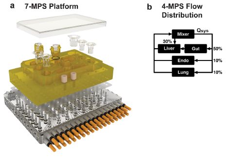
Frame a (left side) shows a device, dissembled into layers. (MPS = microphysiological system(s).) The upper layer holds several specialized cell-culture "cups". This device has seven such cups. Three of them are clear at the upper right; the others are in the middle, where they almost blend into the yellowish plastic support.

You can see that the cups are different sizes. It you think of the cups as being about one centimeter diameter, you will get an idea of the size of the device. Each cup holds one MPS -- or "organ". There are devices with 4, 7, or 10 organs in this article.

The rest of the device is plumbing.

Frame b (right side) gives an example of what the plumbing accomplishes. This frame is for a simpler device, with only four organs. ("Endo" = endometrium.) The device is programmed to deliver fluid to the organs as shown here. The details are not important for now; the point is that fluid flows can be set. This includes flows from one organ to another.

This is part of Figure 2 from the article.

That establishes the general idea of the system. The organs are maintained separately, but interact through the plumbing.

What happens? As a start, the scientists measured one property of each organ over time. The following figure shows some results, as examples...

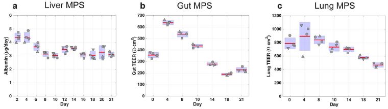
The graphs show results for three of the organs in a 7-organ device.

The details don't matter much. This is early work, and what's important here is that they are beginning to establish such systems.

In general, you can see that each organ was maintained as functional over the three weeks of measurement. The quality varied. I do note that the consistency of the liver measurement was much better here than with the 4-organ device.

For liver, the measurement is albumin production. For the others, it is the TEER = trans-epithelial electrical resistance, a measure of the quality of the surface.

The other organs in this 7-organ device were: endometrium, heart, pancreas, and brain.

The 10-organ device included all those, plus: skin, kidney, and skeletal muscle.

This is part of Figure 4 from the article. The full figure contains results for each of the seven organs in this device. The article also contains similar figures for each organ in the 4-organ and 10-organ devices.

The goal here is to show how the scientists are developing multi-organ lab chips, or "physiome-on-a-chip", with interactions between the organs. The article is complex, because the system is complex. Each "organ" has to be developed, and the multi-chip platform is a complex device integrating complex biological systems. There is considerable empirical development of operating parameters. In some tests, cells were replaced after problems occurred. Overall, it is progress. The authors say that theirs is the first such system to integrate seven organs.

It's an interesting approach; the results show that such devices are possible.

News stories. The following two stories are similar, but have quite different figures.
* DARPA-funded 'body on a chip' microfluidic system could revolutionize drug evaluation -- Linked by microfluidic channels, compact system replicates interactions of 2 million human-tissue cells in 10 "organs on chips," replacing animal testing. (Kurzweil, March 19, 2018.)
* "Body on a chip" could improve drug evaluation -- Human tissue samples linked by microfluidic channels replicate interactions of multiple organs. (A Trafton, MIT News, March 14, 2018.) From the lead institution.

The article, which is freely available: Interconnected Microphysiological Systems for Quantitative Biology and Pharmacology Studies. (C D Edington et al, Scientific Reports 8:4530, March 14, 2018.)

Background posts include:
* Human heart organoids show ability to regenerate (May 2, 2017).
* How much would it cost to make a brain? (November 1, 2015). Considers drug testing using lab mini-brains.
* Autism in a dish? (September 4, 2015). Develops and compares lab tissue from multiple individuals.

Lab-on-a-chip -- but no biology: Using music to control a machine (October 17, 2009).

Also see: Using lab-grown organoids in medical treatment (May 3, 2021).

April 11, 2018

Growing meat without an animal?

April 11, 2018

Mankind consumes a lot of meat. Would it be possible -- or practical -- to make meat without growing animals? It's an intriguing question.

Biologists have been growing cells in lab-scale cultures for decades. And they have been learning how to grow organized multi-layer structures, sometimes called 3D cultures. In some cases, tissues have been grown in culture that are suitable for transplantation back into an animal. Growing meat, which is typically muscle tissue, under such conditions, might seem to be just one example of such an application.

A news feature-type article in the magazine of a scientific society gives a good overview of the field. It discusses the motivations for trying to make "cultured meat", and the barriers to doing so. It's worth reading as an introduction and status report.

News feature, which is freely available: Clean meat. (L Cassiday, INFORM, February 2018.) INFORM is a magazine from the American Oil Chemists' Society (AOCS). INFORM is itself an acronym, describing the science content. The article includes an extensive list of references, many of them to recent scientific articles.

You can also download the entire issue as a pdf file. Go to the INFORM archive, and scroll down to the February 2018 issue. There is a link there to download the issue.

Thanks to Borislav for sending the article.

* * * * *

More about cultured meat:
* Added June 24, 2023. Briefly noted... Cultured meat: the environmental cost (June 24, 2023).
* Added June 22, 2023. Briefly noted... Cultured meat -- using spinach. (May 26, 2021).
* Tuning the protein and fat content of cultured meat (February 2, 2021).

Posts about meat include...
* Why you should not eat larb: A story of trichinellosis -- locally (March 11, 2018). Most recent meat post.
* Sliced meat: implications for size of human mouth and brain? (March 23, 2016).
* The WHO report on the possible carcinogenicity of meat (December 12, 2015). It's important to note that one should not expect the nutritional aspects of cultured meat to be any different than for natural meat. The goal of cultured meat is an alternative process, not an improved process. Of course, it would allow for targeting nutritional issues, by process or genetic modification, as later developments.
* Carnivorous algae -- that hunt large animals (October 7, 2012).

My page Biotechnology in the News (BITN) for Cloning and stem cells includes an extensive list of related Musings posts.

How frequent are volcanic eruptions that are truly catastrophic?

April 10, 2018

Most problems are small. Most earthquakes are small. Most volcanic eruptions are small. But it is the rare big ones that are potentially the most serious. We would like estimates of the chances of big events, but it can be hard to get them.

A recent article looks at the chances of catastrophic volcanic eruptions. It's interesting to see how they approached the problem. There is no basis for theoretical predictions. All we can do is to look at the historical record.

For this work, the authors define a catastrophic eruption as one of magnitude 8 or greater. That corresponds to the ejection of 1000 gigatons (Gt). Such eruptions could have serious effects worldwide.

The magnitude scale used here for volcanoes has nothing to do with the magnitude scale for earthquakes. (However, I suspect that the way it was scaled was intended to make it somewhat similar in result.)

An estimate of the frequency of such "super-eruptions" was published in 2004. That estimate was that such eruptions would occur every 45-714 thousand years.

The following figure shows some of the data behind the new work...

Each frame shows the cumulative count of volcanic eruptions of the specified magnitude over time, for the last 100,000 years (100 kiloyears, or ky).

Start with the bottom frame. It is for major eruptions, those with magnitude above 7.5. (Note that the graph does not quite correspond to the cutoff for "catastrophic" eruptions, which is M = 8. There is a reason for this, but it doesn't really matter much.) You can see that only five such eruptions have been identified; they are labeled. Their occurrence is erratic; given their low frequency, that is of no particular significance. You can also see that there is, on average, one such eruption every 20 ky. (That's every 25 ky if you only include magnitude ≥8.)

Now look at the top frame. Same idea, but for eruptions of a medium magnitude; these are much more frequent. The shape of the curve is perhaps surprising. Wouldn't one expect a linear accumulation of events over the long term? Are volcanic eruptions becoming steadily more frequent, or is something else going on?

Caution... The authors use both "a" and "y" for years, with abbreviations such as ka and ky. They make a distinction... y is for dates, a is for intervals. That is, an event might be dated to, say, 100 ky ago. And the average interval between events would be, say, 20 ka. I don't think the distinction matters much, or that there will be any confusion if you mix them up -- other than wondering why they use two symbols for the "same" thing.

This is part of Figure 2 from the article. The full figure shows more magnitude ranges. The additional frames are similar to the top frame above.

The authors suggest that the accelerating pace seen in the top frame above is due to bias in the records. Note that one big change in slope was about 40,000 years ago. This is not about recordkeeping, but about our ability to recognize old volcanic events. It's plausible that older events are harder to detect. The authors take this under-recording into account in their current analysis. It is an example of the subtleties they uncover, helping them to adjust the observed record.

When they run all the numbers, their best estimate of the average interval between catastrophic eruptions is about 17,000 years. Their estimate is a lot less than the earlier one; that's due to the greater number of events in the database, as well as to how they do the estimate. The estimated interval is getting close to the time span of recorded history. (The estimate has considerable uncertainty, of course; the 95% confidence limits are 5-48 ky.)

In one sense, there is nothing here that is particularly important. We have no basis for predicting such events, and the probability of one happening this year is low. Nothing in the analysis changes any of that. However, the display of data is of some interest, and it is interesting to see how the authors attempt to analyze the data. Overall, a "fun" little article.

News story: Time between world-changing volcanic super-eruptions less than previously thought. (University of Bristol, November 29, 2017.) From the University.

The article: The global magnitude-frequency relationship for large explosive volcanic eruptions. (J Rougier et al, Earth and Planetary Science Letters 482:621, January 15, 2018.)

Posts about volcanoes include:
* Rise of the Roman Empire: role of an Alaskan volcano? (July 28, 2020).
* Aerosols and clouds and cooling? (August 27, 2017).
* What caused the dinosaur extinction? Did volcanoes in India play a role? (April 13, 2015).
* VPOW (July 14, 2010).

Posts about major earthquakes include:
* Are large earthquakes occurring non-randomly? (February 10, 2012).
* The great Tonga earthquake: how many quakes were there? (September 12, 2010). Hm, could this happen for volcanoes? Would it be possible to have a great eruption, and no one notices?

More catastrophes: Could we treat COVID by driving it to an error catastrophe? (June 30, 2020).

The fetal kick

April 7, 2018

Briefly noted...

The mammalian fetus moves during development. For humans, motions start at about 10 weeks of development, and are usually evident to the mother by about 17 weeks. Fetuses that do not move normally often end up showing abnormal development; that is, fetal movements are part of development. In some sense, fetal movements are like exercise, and play a role in developing the skeleton.

It is now possible to observe fetal movements, using magnetic resonance imaging (MRI) -- a procedure called cine-MRI.

A new article examines many sequences of human fetal movement. The striking feature of the article is the "movies".

The following movie file, at the journal web site, illustrates several kick sequences, from human fetuses of various ages.
Movie 2. It is an animated gif, so it loops, but is fundamentally only a few seconds. Individual kick sequences are 2-4 seconds. (The gif file itself is almost 15 MB, so be patient if you have a slow connection.)

The article contains some analysis of the data. The authors develop models that allow them to estimate the forces involved, including the force on the wall of the uterus. They show graphs of the stresses and strains over the course of pregnancy. It's pioneering work, building on the pioneering measurements. But it is also very limited at this point. The news stories introduce this aspect of the work.

There is also discussion of the implications. The article starts with an overview of what is known about fetal movements, and the possible implications of absent or aberrant movements.

"This research represents the first quantification of kick force and mechanical stress and strain due to fetal movements in the human skeleton in utero, thus advancing our understanding of the biomechanical environment of the uterus." (From the abstract.)

News stories:
* Monitoring fetal movements helps detect musculoskeletal malformations. (B Yirka, Medical Xpress, January 24, 2018.)
* First study of its kind shows how foetal strength changes over time. (C Brogan, Phys.org, February 2, 2018.)

The article, which is freely available: Stresses and strains on the human fetal skeleton during development. (S W Verbruggen et al, Journal of the Royal Society Interface 15:20170593, January 2018.)

More fetal imaging... Imaging of fetal human brains: evidence that babies born prematurely may already have brain problems (March 10, 2017).

More things uterine...
* Involvement of the non-pregnant uterus in brain function? (February 11, 2019).
* Lamb-in-a-bag (July 14, 2017).
* Cannibalism in the uterus (May 31, 2013).

Observing inside animals with an improved bioluminescence system

April 6, 2018

Imaging is an important part of modern biology. Medical imaging techniques such as CAT scans and MRI are examples, which involve some fancy technologies. But they also require that the subject stay still. What if we could image the inside of an animal as it wandered around its cage?

One approach is to use bioluminescence. Most animals are not naturally bioluminescent, but one can make lab animals that carry the gene for the light-making enzyme. Then we could just watch the animals' light emission.

A recent article reports an interesting development that could make such imaging more practical. The following figure presents one key step.

Terms: Luciferase is an enzyme. It acts on a substrate called luciferin. The resulting reaction emits light. But caution...

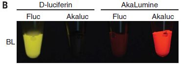
The figure shows the bioluminescence from four systems. They have various combinations of substrate (labeled in top row) and enzyme (second row).

The first tube (at left) shows a natural system: firefly luciferase (Fluc) acting on the common luciferin.

The last tube (right) shows the system developed in the new work. It uses a new enzyme (Akaluc) and a new substrate (AkaLumine). Development of the new enzyme is the heart of the current work; the new substrate had been developed earlier.

The results show that the new system is different from the original system in two ways: brighter and redder.

Tissue transmits red light better than other colors. So the new system is better suited for use within animals both because it is intrinsically brighter, but also because it emits a color that is more suitable for this use. (In fact, much of the emission is in the infrared (IR), where transmission is even better.)

The other two tubes are for hybrids between the two systems, such as old substrate with new enzyme. They show little.

BL at the left of the figure means bioluminescence.

This is part of Figure 1B from the article.

Here is an example of the use of the new system with an intact animal.

The animal was injected with a small number of cells that express the new luciferase enzyme (Akaluc). In this case, the injection was about 5 millimeters into the brain of a marmoset (a small monkey).

To prepare for a set of measurements, a solution of the luciferin was injected into the abdominal cavity. In this case, that was about a year following the injection of the cells capable of making the luciferase enzyme.

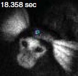
The figure shown here is actually a composite of two types of images that were obtained, using the same electronic camera. One is an ordinary optical image, showing the animal. The other is the bioluminescence. But that is not shown directly. (Remember, it is red, actually peaking in the IR). The camera records the bioluminescence signal, processes it, and displays it with a false color that represents the intensity. That's why the red emission is represented here by blue -- denoting a medium amount of the red light. (There is a color bar in the full figure translating the color shown to the intensity.)

Don't see the bioluminescence signal? It's a small blue circle, about the size of the letter c in the label at the top. It's on the forehead, about half way between the ears.

This is part of Figure 4D from the article.

A feature of the image above is that it was obtained on a "free" animal -- neither held down nor anesthetized. And that's the point. The method developed here can be used to observe what is going on inside an animal's body as it goes about its ordinary activity. That could be a useful tool.

Movies. In fact, the image above is a frame from a movie sequence. There are three movie files posted at the journal web site along with the article. Without getting into the details, each shows an example of light emission from the head of an animal labeled with the new bioluminescence system. The first two show mice; the third shows the marmoset seen above. I encourage you to check at least one of them. (Each is about a half minute; no sound.)

News story: In living color: seeing cells from outside the body with synthetic bioluminescence. (Phys.org, February 22, 2018.)

* News story accompanying the article: Imaging: Unnaturally aglow with a bright inner light -- A bioluminescent system enables imaging single cells deep inside small animals. (Y Nasu & R E Campbell, Science 359:868, February 23, 2018.)
* The article: Single-cell bioluminescence imaging of deep tissue in freely moving animals. (S Iwano et al, Science 359:935, February 23, 2018.)

More on bioluminescence:
* Milky seas: now observable from space (September 27, 2021).
* Xystocheir bistipita is really a Motyxia: significance for understanding bioluminescence (May 9, 2015).

There is a section of my page Internet resources: Chemistry - Miscellaneous on Chemiluminescence. It includes a list of related Musings posts.

A post that is a reminder about the importance of staying still for an MRI scan... Dog fMRI (June 8, 2012).

Another way to see what is going on inside the head of an animal is to remove the top and look inside... A microscope small enough that a mouse can wear it on its head (November 12, 2011).

April 4, 2018

Should we geoengineer glaciers to reduce their melting?

April 4, 2018

Glaciers are melting at an increased rate because of global warming. That leads to rising sea level, which can impact people near coasts around the world.

What if we tried to reduce glacier melting, by cutting off the local heat source or supporting the ice shelves that hold back glacier movement? Those are among the proposals put forward in a recent "Comment" article in Nature.

Apparently, not much thought has been given to such an approach to mitigate one aspect of global warming. The authors' goal is to put the topic on the table. If nothing else, the article is interesting in discussing how glaciers melt; in fact, the authors emphasize the importance of improving our understanding of glaciers as part of considering intervention. They have some specific proposals, and they discuss pro and con aspects.

It's an intriguing and provocative article.

"Comment" article, which is freely available: Geoengineer polar glaciers to slow sea-level rise. (J C Moore et al, Nature 555:303, March 15, 2018.)

A post about sea level changes, including the contribution from glaciers melting: Climate change and sea level (October 2, 2017).

A post about the more commonly discussed type of geoengineering, with the goal of changing the atmosphere: Geoengineering: the advantage of putting limestone in the atmosphere (January 20, 2017). Links to more.

The glaciers of particular concern here are in Greenland and Antarctica. Posts about other things from those lands include...
* Is Arctic warming leading to colder winters in the eastern United States? (May 11, 2018).
* What do microbes eat when there is nothing to eat in Antarctica? (April 2, 2018). That's the post immediately below. Links to more.
* Inuk, a 4000 year old Saqqaq from Qeqertasussuk (March 1, 2010). Links to more from the Arctic.

More ice: Ice in your diamond? (April 23, 2018).

What do microbes eat when there is nothing to eat in Antarctica?

April 2, 2018

They eat the air, according to a new article.

Antarctica is a harsh place. However, there are diverse microbial communities, with no obvious source of food. We commonly think of photosynthesis as the primary energy source for most life on Earth, with some specialized communities using chemical energy, such as that from thermal vents in the oceans. These Antarctic microbial communities seem to have extremely low photosynthesis; anyway, it's dark much of the year there.

A recent article explores the basis of life on the Antarctic desert. It uses extensive DNA sequencing -- metagenomics. And it does some biochemical testing.

Here is one of the experiments from the article...

The graph shows CO₂ fixation under various conditions for soil samples from two sites in Antarctica.

Focus on the right hand set, from Adams Flat.

The four conditions are shown at the bottom, with their color code. The order of the bars in the graph is the same as the order in the key.

The first two bars (from the left) are for CO₂ fixation in the dark, without or with hydrogen. You can see that CO₂ fixation is higher with H₂; the difference is statistically significant, as shown by the p value (and asterisks).

The next two bars are for similar conditions, but with light. That is, without and with H₂ in the light. The pattern is the same as in the dark.

Now compare the data without and with light. They are very similar. (The p value at the top says they are not significantly different.)

This is Extended Data Figure 4c from the online version of the article.

Those results from Adams Flat suggest that CO₂ fixation is stimulated by H₂, but not by light. That is, the microbes are growing using chemical energy (from H₂) and using CO₂ as their carbon source. They use chemical energy (not light energy) to drive CO₂ fixation.

You can also see that there is considerable variability. And for the other site, Robinson Ridge, there is no clear trend. (However, separation of the Robinson Ridge data by specific site suggests that one of them behaves similarly to the Adams Flat samples.)

What makes the results particularly interesting is that the experiment was done using a level of H₂ typical of the ambient air. Further...
- Direct testing of H₂ metabolism showed that it was consumed at that low level. (H₂ consumption was found even at the lowest temperature tested: -12 °C.)
- Analysis of the DNA in the soils showed that the key enzyme needed for H₂ metabolism, hydrogenase, was present. It was a type of hydrogenase considered high-affinity, able to metabolize low levels of H₂.

The scientists also showed that carbon monoxide was consumed at the level found in ambient air, and that the key enzyme needed for that metabolism, carbon monoxide dehydrogenase, was present.

Bottom line... The article provides evidence that microbes on the Antarctic desert metabolize trace levels of combustible gases in the air. They use these trace gases, H₂ and CO, as energy sources. Both gases are present at quite low levels, but they probably are reliable energy sources -- at least by Antarctic standards.

The bacteria use CO₂ from the air as their carbon source. They use the common C-fixing enzyme Rubisco for that purpose. There is nothing unusual about this step.

The main claim is that the bacteria use the trace gases from the air for maintenance energy. Whether they use these gases for primary growth is an open question.

We should stress that the scientists have not isolated any particular organism with the claimed properties. The metagenomic studies show what genes are present in the population, with some clues about how they might be combined into chromosomes of individual bacteria. The metabolic studies are with soil samples. Thus the article offers hypotheses about what is happening, but there is more to do, and many questions remain.

The authors propose two new phyla of bacteria, based on the work: Eremiobacteraeota (desert bacterial phylum) and Dormibacteraeota (dormant bacterial phylum).

News story: Living on thin air - microbe mystery solved. (Phys.org, December 6, 2017.)

* News story accompanying the article: Microbial ecology: Energy from thin air. (D A Cowan & T P Makhalanyane, Nature 552:336, December 21, 2017.)
* The article, which is freely available: Atmospheric trace gases support primary production in Antarctic desert surface soil. (M Ji et al, Nature 552:400, December 21, 2017.)

A recent post about other bacteria that seem to be having trouble finding food: Nuclear-powered bacteria: suitable for Europa? (March 27, 2018).

Posts about Antarctica include...
* Should we geoengineer glaciers to reduce their melting? (April 4, 2018). That's the post immediately above.
* A bit of IPD -- found in Antarctica (January 13, 2015).
* IceCube finds 28 neutrinos -- from beyond the solar system (June 8, 2014). Nice picture of Antarctica -- a very different scene than the desert of the current work.
* Life in an Antarctic lake (April 22, 2013).
* How were the Gamburtsevs formed? (December 7, 2011).

This post is noted on my page Unusual microbes.

There is more about DNA sequencing on my page Biotechnology in the News (BITN) - DNA and the genome. It includes an extensive list of related Musings posts.

A blood test that detects multiple types of cancer

March 30, 2018

The article discussed here is complicated. It is also very interesting, and potentially important; it has received considerable news coverage. So, let's start with a summary, for perspective... The article presents a blood test for cancer -- a general test, to detect any kind of cancer. The approach is to measure many things. The results are encouraging, suggesting that such a test might be practical and useful. However, this is a very preliminary report, and much work remains to be done.

The test starts with a blood sample. The blood is tested by DNA sequencing. It is now recognized that there is a variety of DNA floating around in the blood -- including DNA from tumor cells. Recent developments in DNA sequencing allow us to find and sequence even very low levels of DNA, almost blindly. For the current use, the scientists focus on a set of genes that often carry mutations in cancers. The idea is that if the person has a cancer with a mutation in one of the common cancer genes, then such mutant cancer DNA will be found in the blood. What they do is to take the blood, and use PCR to amplify any DNA that comes from such cancer genes. They then sequence the PCR-amplified DNA, which is now enriched for cancer genes.

As a preliminary step, they need to choose which cancer genes to look for. They start with databases of cancer genomes, and make a list of specific mutant sequences that are common in cancers. These are sequences worth looking for. They get a list of about 200 possible sequences.

How many should they actually use? Use too few, and they will miss some cancers. But the more genes one looks at, the more expensive the test. The following experiment explores that trade-off.

The test is a computer analysis, but it uses real genome data. What the scientists do is to test a database of genomes from cancer patients, and see what the detection frequency would be if they used various numbers of test sequences.

The following figure illustrates what they find...

The three graphs show the chance of detecting the cancer (y-axis) vs the number of sequences -- or "amplicons" -- tested (x-axis). The term amplicon reflects the role of the PCR amplification. The x-axis is labeled here for the middle frame; it is the same for all frames.

Results are shown here for two specific types of cancer (ovary and liver), as well as the overall analysis for all eight types of cancer examined (left-hand panel).

Start with the middle panel, for ovarian cancer. The solid line shows that the chance of finding a cancer increases as they test more sequences. The important point is that the curve gradually levels off, and reaches a plateau at about 60 sequences tested. Without quibbling about the exact number... It is good to test 60 sequences, but there is little value in testing more than that.

The right-hand panel is a similar analysis for liver cancer. The percent of cancers detected is lower than for ovarian cancer, but the shape of the response curve is the same. In particular, 60 sequences is once again a good cutoff.

The full analysis reported in the article includes six more types of cancer. The pattern is similar for all, as illustrated by the two just discussed.

The left-hand panel is a summary over all eight types of cancer studied. Qualitatively, the graph is similar to the other two. The big point is that using about 60 sequences is a good compromise; little is gained by using more. The scientists settled on a set of 61 test sequences.

Each graph also contains a single point. It is at x = 61 amplicons. And the y value is just above the line we have been discussing. The point is based on an independent test with about a thousand cancer patients. Blood samples were tested, using the set of 61 test sequences. In each case shown here, the results were a little better than predicted from the solid line. (In fact, that was true for each type of cancer in the full study -- except one, for which the solid line was already very near 100%.)

That point at x = 61 supports that the test with 61 test sequences detects a high percentage of cancers of various types.

This is slightly modified from the top row of Figure 1 of the article. The full figure also shows the results for six more types of cancer. I have added some labeling for the x-axis of the central panel here; it is the same for each panel.

So far, we have a test done with a single blood sample. It detects a variety of cancers, with about 70% effectiveness overall.

The test builds on recent developments. It makes use of the extensive databases of cancer genomes. And it makes use of low-cost DNA sequencing; that is intrinsic to the test, as well as being behind the databases.

The scientists added eight cancer protein markers to the test; these were tested using standard immunoassays of the same blood sample. These increased the detection percentages. They also added 31 additional protein tests, as follow-up. With these, they were now able to address the question of cancer type. As before, the results vary by type of cancer, but are in the same range as above.

The DNA sequence testing, alone, yields no information about the type of cancer. The gene sequences tested are mutated in cancers generally; they are not specific to types of cancer.

What do we make of the test? It's an interesting development. It is providing information that is not currently easily obtained. Some of the cancer types studied here do not now have any early-detection system. But this is an early step. The authors do not claim this is a test ready for widespread use at this point.

Here are a couple of the issues for this test...

Cost. The authors estimate the test would cost about $500 (USD). Is that expensive or not? Not an easy question. It's actually in the range of many medical tests, though certainly more expensive than many routine tests. Of course, along with cost, we need to consider benefit. A simple screen for early-stage cancer would have tremendous benefit. The article has some information about the stage at which cancer becomes detectable by the proposed test; it's mixed. For now, the point is that cost (and benefit) must be carefully considered.

False positives. Tests such as this have two types of error. One is missing some cases; we call these false negatives. Above, we noted that the test finds about 70% of the cancers; it's missing a lot, but it is detecting many cases that would be missed otherwise. That may be useful progress. Tests may also find things that aren't real; we call these false positives. The article suggests that the rate of false positives here is about 1%. That may seem good, but even a low rate of false positives can be a problem.

To illustrate the problem of false positives... Imagine we have a test with 1% false positives. That sounds good. But let's use the test on the general population with a condition that occurs with 1% frequency. We test 100 people. We detect one case, and we get one false positive (statistically). That is, half the "hits" are false positives. Both of those will have to undergo further testing. Adjust the numbers a little, and you can see that broad screening for rare conditions can yield mainly false positives. Of course, the problem of false positives becomes less as the real incidence increases. False positives are less of an issue when screening populations at high risk (i.e., with higher incidence). There is no simple answer to what level of false positives is acceptable; it depends on the details of the situation, but it is a point that must be considered, especially in tests intended for broad screening.

Overall, as we have already noted, the article is an interesting step toward a general test for cancer.

The test is called CancerSEEK.

News stories:
* Simple blood test detects eight different kinds of cancer -- 'Liquid biopsy' technique looks for genetic mutations and proteins linked with tumours. (H Ledford, Nature, January 18, 2018.)
* Single Blood Test Screens for Eight Cancer Types -- Provides unique new framework for early detection of the most common cancers. (Johns Hopkins Medicine, January 18, 2018.) From the lead institution. It is a good overview of the work. As expected, perhaps, from the source, it is not so good at critical analysis. The following two news sources are better at that aspect.
* Expert reaction to paper on potential non-invasive blood test for multiple types of cancer. (Science Media Centre, January 18, 2018.)

* News story accompanying the article: Cancer: Cancer detection: Seeking signals in blood -- Combining gene mutations and protein biomarkers for earlier detection and localization. (M Kalinich & D A Haber, Science 359:866, February 23, 2018.)
* The article: Detection and localization of surgically resectable cancers with a multi-analyte blood test. (J D Cohen et al, Science 359:926, February 23, 2018.) Check Google Scholar for a freely available pdf of a preprint.

Another example of analyzing DNA that just happens to be in the blood: Genome sequencing of a human fetus (August 25, 2012).

More blood testing: Should we screen the blood supply for Zika virus? (May 20, 2018).

My page for Biotechnology in the News (BITN) -- Other topics includes a section on Cancer. It includes an extensive list of relevant Musings posts.

There is more about DNA sequencing on my page Biotechnology in the News (BITN) - DNA and the genome. It includes an extensive list of related Musings posts.

March 28, 2018

Nuclear-powered bacteria: suitable for Europa?

March 27, 2018

There is water on the Jovian moon Europa. There is almost certainly an ocean, under the surface. Is there life? What would be its energy source? There is no sunlight deep underground. Chemical energy? Perhaps. Or maybe nuclear energy.

A recent article examines the possibility that life on Europa might be powered by nuclear energy.

Here's the idea...

Start at the lower left. There is some UO₂. That's the mineral uraninite -- a common mineral in the Solar System. What's important is that it is radioactive, and gives off gamma rays -- which are shown emanating from the mineral. (Isotopes of thorium and potassium also contribute γ-rays.)

The γ-rays break some water molecules into pieces: the hydrogen and hydroxyl radicals. (Careful... Not the ions, but the radicals.) That step is called radiolysis -- of water, in this case.

Two hydroxyl radicals can join together to form hydrogen peroxide, H₂O₂. Two hydrogen radicals can join together to form hydrogen molecules, H₂. These two products are shown to the top and to the right, respectively.

The overall result of those steps is to convert ordinary water molecules into hydrogen peroxide plus hydrogen -- an oxidant and a fuel.
2 H₂O --> H₂O₂ + H₂.
That sounds hard. It is. It took nuclear energy to do it.

Continuing... There is some pyrite, FeS₂. A sulfide mineral. Hydrogen peroxide (or the hydroxyl radical itself) can oxidize the pyrite -- the sulfide -- to make sulfate, SO₄^2-.

And finally, the biology. It's well known than some bacteria can grow by oxidizing hydrogen with sulfate. And that's what the bug at the right does. The bug itself carries out ordinary biochemistry, but its substrates are present because of the radiolysis of water promoted by the γ-rays from the radioactive uranium.

This is Figure 1 from the article.

Put all that together, and you have a nuclear-powered bacterium. In a very real sense, the bacteria are nuclear-powered, but it is also true that they are ordinary bacteria, doing ordinary biochemistry. It is the overall biogeochemical picture that makes us characterize the bacteria as nuclear-powered, not any special biochemistry.

Think about... If your electric utility uses nuclear energy, you don't get uranium in your electrical lines. The nuclear reaction just provides the energy for the first step: heating water in the case of a nuclear reactor making electricity. The electricity you get is ordinary electricity. Similarly here, the nuclear reaction just provides the energy for the first step.

In fact, that pathway shown above was proposed for a bacterium discovered in South Africa a decade ago, Candidatus Desulforudis audaxviator. (The lead word there means that we have a proposed name.) The organism was growing -- alone -- deep in a gold mine. As best we can tell, it is growing just as suggested in the figure above. It is a nuclear-powered bacterium -- on Earth.

The current article builds on that model, and explores whether it might hold on Europa. In particular, the article does quantitative modeling, using estimates of the relevant parameters. The general conclusion is that it seems reasonable. That doesn't seem a big surprise, given that we have such an organism on Earth. But the extension to Europa is at least provocative. It raises the possibility, even plausibility, that life on Europa is nuclear-powered. It also provides some guidance as to things we might want to measure on Europa.

News stories:
* This Strange Species That Lives Off Nuclear Energy Is Like Alien Life on Earth. (M Starr, Science Alert, February 26, 2018.)
* Brazilians create model to evaluate possibility of life on Jupiter's icy moon. (J T Arantes, Agência FAPESP, February 21, 2018.) From the São Paulo Research Foundation, a funding source for the current work; FAPESP is an acronym based on their Portuguese name. Overall, this is an excellent overview of the article, with context and implications. (But note that the news story does mix up ions and radicals at one point.)

The article, which is freely available: Microbial habitability of Europa sustained by radioactive sources. (T Altair et al, Scientific Reports, 8:260, January 10, 2018.)

More on Europa:
* Does Europa glow? (May 10, 2021).
* Europa is leaking (February 10, 2014).

The nuclear-powered bacterium Desulforudis audaxviator was noted on my Unusual microbes page, under Briefly noted; scroll down to A lonely bug. As you can tell from that header, another property is emphasized.

The biological use of sulfate as an oxidizing agent was noted in the post: The miracle of Methylomirabilis (May 10, 2010).

and... Microbes that make elemental carbon (November 27, 2021).

More about the hydroxyl radical: Spontaneous formation of hydrogen peroxide from water (October 26, 2019).

Other bacteria that seem to be having trouble finding food:... What do microbes eat when there is nothing to eat in Antarctica? (April 2, 2018).

More about the possibility of life in the Jovian system: Is there enough water in the clouds of Venus to support life? How about Jupiter? (August 7, 2021).

Added February 13, 2024. This post is listed on my page Introductory Chemistry Internet resources in the section Lanthanoids and actinoids.

Genetic clues: Why some monkey species don't get "AIDS" upon infection with the immunodeficiency virus

March 26, 2018

Briefly noted...

HIV, the human immunodeficiency virus, causes the disease called AIDS. A related simian virus, SIV, acts similarly in some monkeys.

Some types of animals, and some individuals, don't get sick from the virus. In some cases, they are resistant to the virus: the virus doesn't grow in the animal. This is easy enough to understand. But in some natural infections, a monkey species does not get sick from SIV, despite the virus replicating quite well. Although there is no problem with the general idea of a virus that replicates but does not cause disease, it is not known how an immunodeficiency virus grows well without causing an immunodeficiency.

The sooty mangabey, Cercocebus atys, is an example of a monkey species that does not get sick from SIV, despite a high viral load. A recent article reports a genome sequence for the sooty mangabey. Analysis of that genome, and comparison with the genomes of other primates, offers some clues about why the animal does not get sick. In particular, the article uncovers some intriguing differences in genes of the immune system between rhesus macaques and sooty mangabeys. Both monkeys support good replication of the SIV, but only the former gets sick from it.

These are leads that need to be followed up, to see whether any of the observed differences can explain the different outcomes of SIV infection. It's typical of such genome survey projects... they find candidate genes, but do not give answers.

News story: Researchers find clues to AIDS resistance in sooty mangabey genome. (Medical Xpress (Emory University), January 3, 2018.) Includes a nice picture of a sooty mangabey. (You can see the soot.) (The news story originally included is no longer available. This is a replacement.)

The article, which is freely available: Sooty mangabey genome sequence provides insight into AIDS resistance in a natural SIV host. (D Palesch et al, Nature 553:77, January 4, 2018.)

An earlier HIV post that notes SIV: How HIV destroys the immune system (March 3, 2014). (This post also offers an explanation for why some monkeys do not get sick from the virus. That was based not on the articles, but on a talk I heard. The gene discussed there is not mentioned in the current article.)

My page for Biotechnology in the News (BITN) -- Other topics has a section on HIV. It includes a list of related posts.

Another recent post with genome sequencing generating leads... Ear lobe genetics: more complicated than you thought (March 23, 2018). The current post starts at an earlier step, simply generating the first genome for an organism.

There is more about genomes on my page Biotechnology in the News (BITN) - DNA and the genome. It includes an extensive list of related Musings posts.

How old is Venice, Italy? Evidence from peaches

March 24, 2018

A peach pit.

It is a peach pit with a story to tell.

This is from Supplement #2 with the article.

The city of Venice, Italy, is perhaps most famous for its canals. Venice was built in a lagoon, using what we would now call landfill. It also has a very famous church, Basilica di San Marco (Saint Mark's Basilica), on the plaza known as Piazza San Marco.

How old is Venice? That we don't know. The early history of Venice is less studied than that of most famous cities. Because it is basically an underwater city, Venice is not a good site for archeologists. Some legends date it back to the Roman empire, but there really is no evidence for that early start. Others suggest that it dates to the 9th century AD, the time of famous developments. For example, the original Saint Mark's Basilica was built starting in the year 828. (The current cathedral dates from the late 11th century.) The suggestion is that it all blossomed at once.

A new article points to an origin of Venice around 700 AD. The article uses the principle that a city must be as old as its oldest known peaches.

Some data...

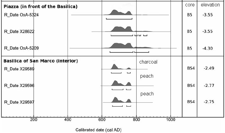
The figure shows the dating of several items from around St Marks Basilica in Venice.

For the most part, it will serve our purposes here to look at the middle part, which shows the dates for the items, as determined by carbon-14 dating. See the date scale at the bottom (x-axis). In general, the dates are in the 600-800 AD range.

What is of particular interest here is that the dates in the lower group have narrower ranges (i.e., less uncertainty) than the ones in the upper group. Those (lower group) are the ones reported in the new article. They include the dates for a piece of charcoal and then for two peach pits. The items were all found under the Cathedral.

Those date curves are odd! Why do they have two peaks? That has to do with how C-14 dating results are calibrated. The measurement itself is logically simple: how much C-14 remains in the sample. But to find the age of the sample, we need to know much C-14 was in the sample originally, and that is a complicated matter. The amount of C-14 in the atmosphere varies, and that affects how much remains. Scientists have done extensive calibration of the C-14 record, commonly using tree rings as the reference. Suffice it to say that certain C-14 measurements actually give ambiguous results upon calibration; that is the case here. The calibration curve is shown in Supplement #2, on the same page as the pictures of the two peach pits, one of which is at the top of this post. Importantly, both peach pits gave the same result. That's good; they were found at almost exactly the same place. Whatever their ages are, they are almost certainly the same.

This is modified from Figure 2 of the article. The full figure shows more data, similar to that of the upper part here. Also, I have added some labeling.

As noted above, one theory is that Venice was started in the 9th century AD. That would mean some time after 800 AD. Previous dating work, such as that in the upper part of the figure above, made a start as late as 800 unlikely, but not impossible. The newer dating, including those two peach pits, reduces the uncertainty, and makes an origin before 800 AD almost certain.

One might wonder... How solid is the connection between peaches and establishment of the city? This is discussed a little in the article. The peach pits were accompanied by other materials likely to be from human activity, and the authors suggest that some of the markings on the pits were made by humans. Further, the elevation of the samples indicates that they were below sea level at the time; that is more evidence that the area had already been filled in, by human activity.

The elevation numbers on the figure are relative to modern sea level. However, the authors have previously done an extensive analysis of sea level changes in the area over two millennia. They claim that the 8th century sea level was about -1.5 m, on the same scale.

It's an interesting article. As so often, we gain knowledge one small piece at a time. Here, two peach pits, found underneath one of the world's most famous churches, are making a small contribution.

News story: Venice Is Much Older Than We Believed. (J Davis, IFLScience, December 15, 2017.)

The article: Beneath the Basilica of San Marco: new light on the origins of Venice. (A J Ammerman et al, Antiquity 91:1620, December 2017.)

Previous posts that mention Venice: none.

Previous posts that mention peaches: none.

In the fine print above, we noted an anomaly in the C-14 calibration curve. That is probably the anomaly discussed in an earlier post: Tree rings, carbon-14, cosmic rays, and a red crucifix (July 16, 2012).

My page of Introductory Chemistry Internet resources includes a section on Nucleosynthesis; astrochemistry; nuclear energy; radioactivity. That section lists Musings posts on related topics, including C-14 dating.

Ear lobe genetics: more complicated than you thought

March 23, 2018

Briefly noted...

It is a common observation that human ear lobes fall into two fairly distinct types: they either do or do not hang loose below the ear. It's often said that the difference is due to a single gene.

For several decades, there have been hints that more genes are involved, but conclusive evidence was lacking.

A new article re-examines the genetic basis of how ear lobes hang. The approach is to collect genome data and ear lobe data. Lots of data. Then let the computer analyze all those data for associations. It's called a genome-wide association study (GWAS). The computer suggested that as many as 49 genes contribute to the ear lobe phenotype.

Some of the genes uncovered here as affecting ear lobes are race-specific. And some play other roles, and may even contribute to pathology.

As usual with such genome scans, the list of suggested genes may not be entirely correct. The approach looks for statistical associations. How the genes are involved is left for further work, and it may turn out that some are just statistical flukes.

The article is a collaboration between academic scientists on five continents, plus the company 23andMe. In fact, of the 74,660 people whose ear lobes were studied here, 64,950 were customers of 23andMe. Other groups studied were small, but ethnically distinct. It's an interesting collaboration between academia and a company that does personal genomics. All this to study ear lobes.

There is more to ear lobes than you thought.

News story: Do your ears hang low? The complex genetics behind earlobe attachment. (Science Daily, November 30, 2017.)

The article, which is freely available: Multiethnic GWAS Reveals Polygenic Architecture of Earlobe Attachment. (J R Shaffer et al, American Journal of Human Genetics 101:913, December 7, 2017.)

Another post on work from 23andMe: The genetics of being a "morning person"? (April 15, 2016).

Another post with genome sequencing generating leads... Genetic clues: Why some monkey species don't get "AIDS" upon infection with the immunodeficiency virus (March 26, 2018).

And... A gene for insomnia? (February 4, 2023).

GWAS overview: Briefly noted... See #1, on GWAS (November 7, 2018).

There is more about genomes on my page Biotechnology in the News (BITN) - DNA and the genome. It includes an extensive list of related Musings posts.

March 21, 2018

Manganese(I) -- and better batteries?

March 21, 2018

The transition metal manganese (Mn) is rich in chemistry. Even beginning chemistry students are likely to encounter it in oxidation states II, IV, and VII -- as well as the free metal at zero. A few more Mn oxidation states are likely to show up in chem classes. But ask an experienced chemist about Mn(I) (or Mn¹⁺) and you may not get much response.

A recent article claims the first clear characterization of manganese in oxidation state I. The context is a new battery.

The main purpose here is to introduce the novel Mn(I). For context, here are some of the battery results...

The graph shows two battery parameters over a thousand cycles (charge-discharge) of testing.

The red curve (y-axis scale at the left) shows the battery capacity. The blue curve (y-axis scale at the right) shows the coulombic efficiency. Both curves show little change over 1000 cycles.

In particular, the battery capacity drops by only about 5% over this time. That's a good start for battery development.

The coulombic efficiency stays very near 1 (or 100%). That means almost no electrons are being lost to side reactions.

This is Figure 6b from the article.

Of particular interest in this battery is a newly developed electrode material. It is based on Prussian blue, a pigment in which iron ions are complexed with cyanide ions. In the new material, Mn is complexed with cyanide ions.

The Mn is presumably playing a key role in the battery redox cycle, but it isn't obvious exactly how. What are its oxidation states, and what changes during use? To explore such questions, the authors examine the material, from charged and discharged batteries, by a type of x-ray analysis, soft X-ray absorption spectroscopy (sXAS). Here are some results from such an analysis...

The measurement is much like an absorption spectrum with light. The x-axis shows the energy of the photons -- X-rays in this case. The y-axis is the response.

There are two types of curves on the figure. The ones at the bottom (thin lines) are theoretical curves for what would be expected for Mn in different chemical environments. All the other curves are experimental results from batteries. The red curves are for charged batteries; the blue curves are for discharged batteries. (The number tells how many cycles the battery has undergone. For example, "40Ch" means that the battery has undergone 40 cycles and is now charged. Turns out that the number doesn't really matter here.)

Start with the theoretical curves at the bottom. There are separate predictions for Mn depending on which end of the cyanide (CN^-) it is attached to. The green curve is for Mn²⁺ attached to the nitrogen atom. The other curves are for various kinds of Mn ion attached to the carbon atom; these turn out to be the ones of interest. (The material has Mn²⁺ attached to the N, but it doesn't change.)

Mn³⁺(C) should give a peak at about 646 eV. None of the battery samples -- all the curves above those theoretical curves -- show any hint of a peak at that position. That is, this kind of measurement suggests than the Mn³⁺ ion is not involved in the battery.

Now look at the theoretical curve for Mn¹⁺(C). It shows an expected peak at about 643 eV. For convenience, the position of that peak is marked by a vertical dashed line (labeled d, at the top). You can see that all of the battery samples show a signal at that position; it is particularly clear in the charged batteries (red curves).

This is Figure 3a from the article.

The results shown above provide evidence for Mn¹⁺ in this battery. If you look more closely, and compare the charged and discharged samples, you will see some hint of an alternation between Mn¹⁺ and Mn²⁺, but it is not convincing.

The evidence for Mn¹⁺ is interesting. Chemists have speculated about this ion for nearly a century, but there has been no evidence for it. So here we have the first experimental evidence for manganese in the 1+ oxidation state.

The scientists go on and do another experiment, using a new technique. That experiment provides further evidence for the 1+ state, and good evidence for the cycling between Mn¹⁺ and Mn²⁺. It's a pretty figure, but too complex to explain here.

Overall, the article describes an interesting new battery -- and a novel behavior of a familiar chemical element.

News stories:
* Monovalent manganese could enable new batteries. (G Pitcher, New Electronics, March 1, 2018.)
* Manganese's novel chemical state could create more efficient batteries. (V R Leotaud, Mining.com, March 4, 2018.) Unusual news source. The lead picture shows a "Manganese oxide rock". Refers to a press release, which is the following item.
* Scientists Confirm Century-Old Speculation on the Chemistry of a High-Performance Battery. (G Roberts, Lawrence Berkeley National Laboratory, February 28, 2018.) From one of the institutions involved in the work.

The article, which is freely available: Monovalent manganese based anodes and cosolvent electrolyte for stable low-cost high-rate sodium-ion batteries. (A Firouzi et al, Nature Communications 9:861, February 28, 2018.) The lead institution is a San Francisco area company called Alveo Energy in the article. It is now Natron Energy.

More about manganese:
* Growing on manganese ions as an energy source (September 15, 2020).
* Photosynthesis that gave off manganese dioxide? (July 21, 2013).
* Penidiella and dysprosium (September 11, 2015). Actually, the results reported here for Mn were negative, but it is the only other post I found about Mn. And it is an interesting post.

Another post about a novel oxidation state: Iridium(IX): the highest oxidation state (December 14, 2014).

Previous post on batteries: Making lithium-ion batteries more elastic (October 10, 2017).

Next: A low-temperature battery (July 29, 2018).

I have listed this post on my page Internet Resources for Organic and Biochemistry under Energy resources. It includes a list of some related Musings posts.

Making wood stronger

March 19, 2018

The following figure provides some perspective. It shows the strength of several materials.

The first four bars (dark; to the left) are for some metal alloys that are noted for high strength. The next bar (blue) is typical of natural wood. The right-hand bar (red) is for the wood product reported in a recent article; that product is called densified wood.

You can see that the natural wood is weaker than any of the metals shown. However, the modified wood product is not only stronger than the original wood, but stronger than the metals.

The "strength" reported here is the specific tensile strength. It relates to the height of a column of the material that can support its own weight. A column of the modified wood could be about four times taller than a column of the natural wood before collapsing of its own weight. The article reports various types of strength measurements. You will see different numbers for the improvement; they are for different types of measurements.

This is part of Figure 1 from the article.

What is this stuff? What is "densified wood"? It is wood that has been made more dense. How do you make wood more dense? Squeeze the air out of it. There is more to it, but that really is a key step.

Here is what the two woods look like...

These are scanning electron microscopy (SEM) images of the two woods.

Natural wood at the top (frame b); densified wood at the bottom (frame e).

It is clear that the open spaces of the natural wood are gone in the densified wood.

Note the scale bars. The image for the densified wood is at a higher magnification than the one for the natural wood. At the same magnification, the densified wood would look even better!

This is from Figure 2 from the article.

The idea of making wood stronger by removing the air is not new. What's new is that the scientists here have succeeded in actually making a stronger product. Their process has two steps. First, they do a chemical treatment, which removes some of the non-cellulosic materials. Then they do the compression step. The results above, the appearance and the strength data, show that they have achieved the goal.

Wood is very light. The densified wood is about three times more dense than the natural wood -- but still less dense than aluminum.

Is an automobile made of wood in our future? It is a reasonable question; strong lightweight materials deserve attention.

News stories:
* Strong as steel and lightweight? Must be superdense wood. (A Micu, ZME Science, February 8, 2018.) Includes the ballistics test.
* New process makes wood stronger than many titanium alloys. (L Donaldson, Materials Today (Elsevier), February 22, 2018.)

* News story accompanying the article: Materials science: Wood made denser and stronger. (P Fratzl, Nature 554:172, February 8, 2018.)
* The article: Processing bulk natural wood into a high-performance structural material. (J Song et al, Nature 554:224, February 8, 2018.)

More about wood strength:
* Transparent wood (March 6, 2021).
* Building with wood: might it replace steel and concrete? (June 14, 2017).
* At what wind speed do trees break? (April 2, 2016).

More about materials...
* Artificial wood (November 3, 2018).
* The strongest bio-material? (May 30, 2018).

More about wood density: Better violins through better fungi? (March 4, 2013).

Diabetes: types 1, 2, 3, 4, 5

March 16, 2018

Diabetes is commonly classified as type 1 or type 2. Type 1 diabetes is characterized by loss of insulin production, because of an auto-immune reaction. In type 2 diabetes, insulin is present but ineffective. These two types of diabetes are treated differently.

Most adults with newly-diagnosed diabetes have type 2. But it has long been clear that type 2 diabetics are a heterogeneous group. They respond differently to treatment, and have different outcomes. Is it possible that we should be recognizing more than two types of diabetes?

A new article proposes a system for classifying diabetes into five types, or "clusters" as the authors call them.

The following figure shows the classification of nearly 9,000 cases of diabetes in adults -- using both the traditional and proposed systems.

Part A (top) shows the cases classified by the traditional system. Part B (bottom) shows the same cases classified by the proposed system.

The two small sectors at the top of part A, together, are for type 1 diabetes. They total 6.4%. The rest, the big sector, is type 2 diabetes, about 94%.

With the proposed system (Part B, bottom), there is a sector of 6.4% at the top; this substantially corresponds to the type 1 diabetes in part A.

The big difference is that the large sector for type 2 diabetes in A is now subdivided into four parts. We now have five types of diabetes with the proposed system.

This is part of Figure 1 of the article.

How did the scientists come up with this new classification system, and what does it mean? The first part of that is straightforward. They fed huge amounts of data to their computer. The data included measurements on the patients soon after diagnosis, and information about how the disease progressed. Statistical analysis of the data set suggested five clusters of diabetes. Each cluster is based on characteristics of the patients as seen early; the clusters predict how the disease progressed.

The system uses six measurements, all of which can be obtained from a single office visit. The following paragraph describes those measurements. (It is based on the second paragraph of the Comment article by Sladek, but I have added a little and reformatted it.)

The measurements used for the new system:
- Age at diagnosis,
- BMI ( a measure of obesity),
- glutamate decarboxylase antibodies (GADA; to identify patients with autoimmune diabetes; key marker for type 1 diabetes, or for cluster 1 in the new system),
- HbA_1c (glycated hemoglobin, a form of the blood protein modified by reaction with glucose; its level is a measure of blood glucose control),
- homoeostatic model assessment 2 (HOMA2-B (to assess function of the insulin-producing β-cells based on concentration of the insulin C-peptide),
- HOMA2-IR (to assess insulin sensitivity).

The key idea is to use more information to help describe the condition. All of the information used here is readily available. The computer analysis has sorted out some patterns in this larger information set, in the context of relating early parameters of the patient to disease outcomes; that is the basis of the new classification scheme.

The goal is to use the more refined classification to guide treatment. For example... Insulin is usually not part of the initial treatment for type 2 diabetes. However, the proposed system identifies one cluster -- a sub-group of the traditional type 2 -- where insulin should be of benefit. We'll see over time if such predictions from the new system lead to improved outcomes. Along the way, we should develop further understanding of the five types of diabetes. Of course, work using the new system and trying to understand it may well lead to further developments in diagnosing and classifying what is clearly a many-factored disease.

News stories:
* New Way to Classify Adult-Onset Diabetes, Explained. (K Monaco, MedPage Today, March 1, 2018.)
* Five categories for adult diabetes, not just type 1 and type 2, study shows. (N Davis, Guardian, March 1, 2018.)

* Comment accompanying the article: The many faces of diabetes: addressing heterogeneity of a complex disease. (R Sladek, Lancet Diabetes Endocrinology 6:348, May 2018.)
* The article: Novel subgroups of adult-onset diabetes and their association with outcomes: a data-driven cluster analysis of six variables. (E Ahlqvist et al, Lancet Diabetes Endocrinology 6:361, May 2018.)

A loose end... In part A of the graph above, there are two small sectors that we combined as type 1 diabetes. What are these? The smaller sector is full-fledged type 1 diabetes. The larger of those two small sectors is a pre-type-1 condition, known as latent autoimmune diabetes in adults (LADA). The person is still making some insulin, but has the antibodies characteristic of type 1 diabetes, indicating that the disease will presumably progress to full type 1.

* * * * *

A recent post on diagnosing diabetes: Diagnosing diabetes in people of African ancestry: a race-dependent variable (January 3, 2018). The focus here is the glucose-modified hemoglobin, noted above as one of the criteria in the new system.

Next post on diabetes: Diabetes type 1: an immunotherapy to delay onset? (April 20, 2021).

More on diabetes is on my page Biotechnology in the News (BITN) -- Other topics under Diabetes. That includes a list of related Musings posts.

More about insulin: Insulin: role in reproduction in ants (October 2, 2018).

March 14, 2018

The oldest known sick dog?

March 14, 2018

A recent post presented the oldest known dog leash [link at the end]. The interpretation helped us understand the history of the relationship between dog and man.

We now have a new story along the same lines. A team of scientists claim they have found the oldest known sick dog. Once again, the interpretation helps us understand man-dog history.

I should note upfront that I am not particularly convinced by the evidence in this case, though I certainly do not have the expertise to make a good judgment. So, a reminder... there are two parts to any such story: the evidence itself and the interpretation.

With that reservation... It is an intriguing story. The scientists do new analyses of an archeological find, and conclude that it is a burial site with the bodies of two people and two dogs.

One of the dogs was very young; the authors claim that the young dog was sick, with distemper. The scientists also claim that the dog survived with the distemper for many weeks, far longer than would be expected unless it was well cared for. As a result, they suggest that the people must have cared for the dog. Since the dog was young and sick, it was probably of no material value to the people. Caring for it, they infer, was due to empathy -- or some form of emotional bonding.

What is the evidence that the dog had distemper, and had it for an extended time? The authors make the case based on their observations of the teeth. The case is not very clear. (That may be due to my lack of expertise for analyzing teeth for signs of distemper.) I do not want to suggest they are wrong, but merely that I don't follow their presentation of the evidence.

The burial find is of interest in any case. It is the oldest known burial site with man and dog together. But the authors do want to make the point that the humans cared for the dog.

The site is dated to about 14,000 years. Whatever it is that man and dog did together at that time is reflected in this burial site.

The authors are actually rather cautious in their conclusions. Here is an excerpt from the final paragraph. (Morbillivirus refers to the virus for distemper. Bonn-Oberkassel refers to the archeological site.)

"We believe that canine morbillivirus infection is consistent with the pathologies that we observed. We hypothesize that this puppy could have survived only with intensive human care over several weeks. The dog was young and sick, likely was untrained as a result, and thus had no obvious utilitarian value to surrounding humans. Thus, we hypothesize further that the inferred supportive care probably was due to compassion or empathy, without any expectation of reciprocal utilitarian benefits. We suggest that the Bonn-Oberkassel dog provides the earliest known evidence for a purely emotion-driven human-dog interaction."

Bottom line? We note the article and its claim. Over time, people will debate the evidence and the argument. Importantly, further evidence may become available.

News stories:
* Emotional bond between humans and dogs dates back 14,000 years. (Phys.org, February 8, 2018.)
* We care for ill dogs for at least 14.000 years. (A Heuzer, Dogzine, February 9, 2018.) This is the first item from this source to be used in Musings. It is a Dutch web site, and we note that this work is, in part, from a Dutch university. The writing is only fair, but the content is good.

The article: A new look at an old dog: Bonn-Oberkassel reconsidered. (L Janssens et al, Journal of Archaeological Science 92:126, April 2018.)

Background post: The oldest known dog leash? (January 23, 2018).

Making better artificial muscles

March 13, 2018

A recent article presents a new type of artificial muscle. The muscle is quite simple, in principle and practice. It's also quite flexible -- literally and figuratively.

The following figure shows the principle...

The top frame shows the basic structure, side view. There is a flexible sheet (blue line), folded up to zigzag, inside a bag (black line).

The bag is full of a fluid (such as water; gray); note the outlet at the upper left corner.

As fluid is removed from the bag (say, with a pump), the inside pressure (P_in) is reduced. The bag collapses. The folded sheet contracts. The figure shows two steps of collapse and contraction as the pressure is reduced. That's it. That's what a muscle does: contract in response to a signal.

This is Figure 1C from the article.

If that diagram leaves you unsure of what is happening, check out one of the videos listed below to see an actual device in operation. You will see that the design is about as simple as the diagram.

A variety of things can be used as construction materials or the fluid. What matters is making a device that will flex under pressure. Negative pressure -- with the inside of the muscle bag at lower pressure than the outside. Of course, the pump could be programmed. In fact, much of the discussion is in the context of these muscles being part of robotic systems.

These muscles are powerful, exceeding mammalian muscles on several criteria. They are also easy to construct and inexpensive, with less than a dollar's worth of materials each (ignoring the external pump).

It seems likely that this work will be the base of a wide range of further developments.

Videos. This is a story well-told with videos; the article is accompanied by seven of them. They are all nice, clear, and short; some are perhaps even funny. (There is no sound.) You can get to them from the article web page; choose figures. (Oddly, they are not quite all in order.)

I suggest you start with the following two videos; each is about 20 seconds.
* Video 3. The best part of this is the second sequence, lifting the tire. It is a good clear example of the device in action. The first example is less clear, because it is not obvious what the control is. I suspect that the device is being filled and emptied from the top right, and is therefore controlling the finger.
* Video 1. A good view of the muscle itself contracting and expanding, though not doing anything in particular in this case.

Beyond that, just explore the videos. I think you'll find them helpful, and maybe even fun.

News stories:
* Origami-inspired artificial muscles can lift 1,000 times their weight. (A Mandal, News-Medical.Net, November 27, 2017.)
* Origami-inspired artificial muscles outperform human ones. (J Timmer, Ars Technica, November 29, 2017.)

The article, which is freely available: Fluid-driven origami-inspired artificial muscles. (S Li et al, PNAS 114:13132, December 12, 2017.) Note that the title leads to the acronym for these devices: FOAMs.

Among posts on muscles...
* Added May 2, 2023. Artificial exercise, using a robotic device glued to the muscle (May 2, 2023).
* Making better muscles using bacteria -- and inteins (September 17 2021).
* How to clamp down to keep the partner from straying (December 15, 2020).
* Human heart organoids show ability to regenerate (May 2, 2017).
* Caltech engineer turns rat into jellyfish (September 22, 2012).
* Mosquitoes that can't fly (May 3, 2010). In this case, the goal is to prevent muscles from working.
* Prosthetic arms (September 16, 2009). This post also involved a fluid-driven muscle.

Other Musings posts about things you can make for less than a dollar include...
* The paperfuge: a centrifuge that costs 20 cents (April 17, 2017).
* How much would it cost to make a brain? (November 1, 2015).

Why you should not eat larb: A story of trichinellosis -- locally

March 11, 2018

Trichinellosis (or trichinosis) is an infection caused by a roundworm of the genus Trichinella. Traditionally, trichinellosis in humans has been associated with eating undercooked pork. However, with improvements in the industry, the incidence of the infection from commercial pork has fallen to essentially zero in the US.

The worm has not been eradicated; it is merely under control -- excellent control -- in the industry. Sporadic cases due to eating walrus or bear are reported.

With that background, a new report of a cluster of trichinellosis cases near a major urban area of the US is striking.

The basic story seems fairly clear. The cluster of cases all arose from a single social event at which larb was served. Larb is an ethnic dish, with uncooked pork. The source was a wild boar raised on a private farm. There is no suggestion that the cluster represents any failure of the industry or of the inspection system. It is simply an example of the risk from animals not subject to the system. Not remote walrus in this case, but wild pigs, apparently grown not too far from a major urban area.

I highlighted that this was a local story; that is what caught my attention. But the details are not clear, at least in the scientific article noted here.

The article is from the Alameda Country Public Health Department, and from Highland Hospital in its major city, Oakland. Alameda Country, in the metropolitan San Francisco area, is the home of the University of California, Berkeley.

The article does not specifically say where the affected people are from, and I have not checked for other news coverage. The article does identify the farm, which was the site of the event, as being in Northern California.

News stories:
* Disease detectives blame raw, wild boar meat for outbreak. (Food Safety News, March 2, 2018.)
* Eating Raw Meat Is Flunking IQ Test. (A Berezow, American Council on Science and Health (ACSH), March 1, 2018.) Caution: This reads as much like an editorial as a news story.

The article, which is freely available: Trichinellosis Outbreak Linked to Consumption of Privately Raised Raw Boar Meat -- California, 2017. (D Heaton et al, Morbidity and Mortality Weekly Report (MMWR) 67:247, March 2, 2018.) As usual with MMWR, there is a nice Summary in the blue box.

More about pork...
* Cooking pork (June 4, 2011).
* Killer chickens - follow-up (December 9, 2009). Includes some statistics about trichinellosis in the US.

More meat: Growing meat without an animal? (April 11, 2018).

More worms: A long worm with a novel toxin (April 28, 2018).

Which came first: butterflies or flowers?

March 9, 2018

The familiar insects of the order Lepidoptera are butterflies and moths. They drink nectar from flowers, sucking it up through a proboscis.

One hypothesis is that drinking flower nectar is fundamental to the origin of this group of Lepidoptera. That is, by this hypothesis, these Lepidoptera evolved along with flowers.

Evidence? Well, it is hard to come by. The oldest known fossil for this group is about 130 million years old. That fits in the range where many people think flowers first appeared.

A recent article reports much older Lepidoptera fossils...

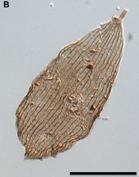
A Lepidoptera wing scale.

Age: about 201 million years.

This is Figure 1B from the article.

Lepidoptera 200 million years old. Some of the wing scales were strikingly like those of modern butterflies. If this is all correct, it would place these Lepidoptera well before the origin of flowers, at least by common estimates. It would then follow that the lepidopteran habit of sucking up fluids with their proboscis must have started with something other than flower nectar.

As you read more about this, you will find considerable uncertainty about the dates. Most obviously, the current article moves the date for oldest known lepidopteran by nearly 80 million years. That is a big move. There is also huge uncertainty about when flowers first appeared.

Therefore, one should take a story such as this in pieces. The article provides evidence for Lepidoptera fossils 200 million years ago. That is much earlier than previously known fossils. This discovery stands on the merits of the characterization of the new samples, including their dating. Assuming it holds up, it is a significant discovery about the history of Lepidoptera. The new discovery may mean that Lepidoptera came before flowers. But that is subject to further discoveries.

We have here an interesting finding; it is part of an incomplete story.

News stories:
* Fossilised Wing Scales Provide Evidence of Triassic Moths and Butterflies. (Everything Dinosaur, January 11, 2018.)
* Rare, delicate fossils show butterflies emerged before flowers did. (M Andrei, ZME Science, January 11, 2018.)

The article, which is freely available: A Triassic-Jurassic window into the evolution of Lepidoptera. (T J B van Eldijk et al, Science Advances 4:e1701568, January 10, 2018.)

Previous post about a Lepidoptera discovery: The Trump moth (January 31, 2017).

Other posts about them include...
* Offering the monarch butterflies milkweed may not be good for them (May 5, 2015).
* Warfare: the tymbal (September 3, 2009).

March 7, 2018

Revealing the alabaster sources of ancient artists

March 7, 2018

Alabaster is a classic material for sculpture. It is a form of calcium sulfate, also known as gypsum.

The term alabaster is actually used for other things, with similar properties. But the current work is about gypsum alabaster.

Chemically, all alabaster is essentially the same. One cannot identify the source of an alabaster sample by chemical analysis. However, different alabaster sources have different isotope ratios for some elements. A recent article shows that the isotope ratios can be used to identify the source used for a particular sculpture.

The following figure illustrates the story...

The graph shows the isotope ratios for two elements found in the alabaster. One is the sulfur that is fundamentally part of alabaster. The other is strontium, an element similar to the calcium of the alabaster, and found as an impurity in the real world.

The dashed ellipses show the range of isotopes found for samples from various quarries the scientists examined. A quick inspection shows that, for the most part, the ellipses for different sites are distinct. That is, the alabaster from each site has a distinctive isotope signature.

Each data point (diamond) shows the isotope results for one sculpture from the 12th through 17th centuries. (They are color-coded by age; see the key at the upper left.)

An example... Look towards the lower right. There is a dashed ellipse labeled UK, East Midlands, Triassic. That refers to a particular source, identified by location and geological age. The dashed region outlines the range of isotope values found for this site. In this case, the Sr ratio (x-axis) is a little over 0.709, and the S ratio (y-axis) is about 13-14 as shown there. (We won't worry exactly how the isotope ratios are expressed; it varies for different cases.) There are also several individual points (diamonds) within that region. Each point is for the isotope ratios for a particular sculpture. The points here match those for this site; it is likely that this site was the source of the alabaster for those sculptures.

Most of the diamonds are within one of the ellipses. That is, the source of the alabaster for most of the sculptures can be identified.

The full work also included analysis of oxygen isotopes.

The analysis of a sculpture requires a speck of the material, about 20 milligrams.

This is Figure 3 from the article.

Overall, the work allowed the identification of the alabaster source for many sculptures, from several European countries over several centuries. That allowed the scientists to infer the trade routes for alabaster. Since there were few written records, this was largely new information. It is an interesting application of isotope analysis. (The conclusions are summarized in the article in another complex figure, Figure 1, with lots of arrows!)

One finding of particular interest was that several of the sculptures could be traced to the region labeled on the figure as France, Alps, N-D-de-Mésage. (Find 14 on the y-axis scale. It's right there.) The importance of this quarry in the alabaster trade had not been appreciated.

News story: Sources of Medieval and Renaissance alabaster. (EurekAlert!, October 23, 2017.)

The article, which is freely available: Competing English, Spanish, and French alabaster trade in Europe over five centuries as evidenced by isotope fingerprinting. (W Kloppmann et al, PNAS 114:11856, November 7, 2017.) Starts with an interesting discussion of the history. (Figure 4 shows an example of an alabaster sculpture, from the 14th century.)

Previous posts about alabaster: none.

Other art materials: What is folium? (July 7, 2020).

Posts that mention strontium:
* Atomic clock measurements of the difference in gravity over one millimeter (May 4, 2022).
* Atoms within atoms? (May 25, 2018).
* Lead-rich stars (August 30, 2013).

My page of Introductory Chemistry Internet resources includes a section on Nuclei; Isotopes; Atomic weights. It includes a list of related Musings posts.

There is more about art on my page Internet resources: Miscellaneous in the section Art & Music. It includes a list of related Musings posts.

A better way to make (the dye for) blue jeans, using bacteria?

March 5, 2018

The following figure, from a new article, lays the groundwork...

At the upper right is the chemical structure of indigo dye.

Next to the indigo is indoxyl. Two molecules of indoxyl join together, in the presence of oxygen, to make indigo dye. That happens spontaneously.

The real problem is making indoxyl. It's not very stable. It tends to form indigo -- and doing that before you apply it to the fabric is not so good.

This is part of Figure 3 from the article. I added the label giving the color of indigo.

How does one make indoxyl? Part a of the figure summarizes the proposed new process. For now, we focus on one piece of that. A key part of the process is a pair of enzymes, which -- overall -- do nothing.

Look just below indoxyl in the figure. There is an arrow, labeled UGT, pointing downward to a more complex chemical. And then there is another arrow, BGL, pointing upwards, back to indoxyl. That more complex chemical below the arrows is indoxyl with a sugar (glucose) attached to it; it is called indican. The UGT enzyme adds glucose to indoxyl; the BGL enzyme takes the glucose off, getting back to indoxyl. Together, the two enzymes end up doing nothing. Well, let's say "nothing".

The point? Indican is a stable chemical. The proposed process makes indoxyl, then stabilizes it by adding a sugar. Indican can be handled by ordinary means. Then, when you want to use it, add the second enzyme and remove the glucose, to regenerate the desired indoxyl. Overall, the pair of enzymes makes no net change. What they do is to provide some control of the process, by stabilizing a key chemical along the way.

The proposed new process is actually a biological process -- a bacterial fermentation -- for making indoxyl, or rather for making indican. The process starts with tryptophan, one of the standard amino acids. Part a of the figure shows the tryptophan being converted to indoxyl, then on to the stable indican. Those are the steps done in the fermentation. The indican is then applied to the fabric, along with the BGL enzyme.

Part b of the figure shows some of the evidence that things are working. It's a simple test: the bacterial culture becomes blue, or not. Blue means there is indigo. It means the process made indoxyl, which spontaneously converted to indigo. As we move from left to right across part b, we see more enzymatic steps...
- At the left, there is no FMO enzyme. That is the enzyme needed to make indoxyl. No FMO means no indoxyl -- and no blue.
- Next, we include the FMO enzyme. Indoxyl is made; it accumulates, and converts to indigo. Blue.
- Next, we also include the UGT enzyme. That converts the indoxyl to indican, the form with glucose. No blue.
- Finally, at the right, we add the BGL enzyme. That gets us back to indoxyl, which spontaneously converts to indigo. Blue.

The glucose is referred to as a protecting group: it is attached to protect the chemical, but then ultimately is removed. The idea of a protecting group is common in organic chemistry; the intentional use here in a biochemical procedure is perhaps more unusual.

That's all about the proposed process, using bacteria to make a stabilized form of indoxyl. What is done now? Indoxyl is made by an ordinary chemical process. It involves chemicals that are now considered environmentally harsh, including a chemical for the step of stabilizing the indoxyl. That is, the proposed process appears to be an environmentally friendly process for getting the dye for blue jeans. Of course, the article here is only an early step; further development is needed to make it economically viable.

News stories:
* Bacteria make blue jeans green. (Phys.org, January 8, 2018.)
* Indigo genes dyeing to make jeans cleaner and greener. (P Ball, Chemistry World, January 9, 2018.)

The article: Employing a biochemical protecting group for a sustainable indigo dyeing strategy. (T M Hsu et al, Nature Chemical Biology 14:256, March 2018.) A very readable article. The work is from the neighboring and oft-collaborating UC Berkeley and Lawrence Berkeley National Laboratory.

More about jeans:
* Using old clothes as building materials? (February 5, 2019).
* Skinny jeans: How tight is too tight? (July 8, 2015).

More about some related dyes: Royal purple E coli (January 19, 2021).

More about dyeing fabric: How to "dye" carbon fiber -- with titanium dioxide (January 20, 2018).

More things blue: Big blue sticks (July 19, 2019).

Some Musings posts about amino acids are listed on the page Internet Resources for Organic and Biochemistry under Amino acids, proteins, genes.

Reducing diesel emissions from ships

March 3, 2018

Ships emit pollution. Of course, they emit much of it out over the oceans, where no one notices -- at least for a while. New standards for ships are planned for 2020. Specifically, ships will be required to use fuel with less than 0.5% sulfur, well below the current limit of 3.5%.

A recent article analyzes the expected effects of ships using cleaner fuel -- for better and worse.

Qualitatively, the cleaner fuel will lead to less particulate emissions. Cleaner air is good for health, but not always for climate change.

The authors' modeling suggests that the switch to cleaner fuel will save about 140,000 lives per year. That's about a third of the estimated deaths due to cardiovascular disease and lung cancer attributed to ships. It is about 2.6% of the global deaths for those conditions.

There is a similar picture for childhood asthma, but with bigger numbers, both absolute and percentage. About 8 million fewer cases, a reduction in cases attributed to ships by about half, and an overall reduction of 3.6%.

That sounds good. But that same reduction in fuel sulfur leads to less sulfur dioxide (SO₂) aerosol. That aerosol serves to cool the Earth. The cleaner fuel will reduce the contribution of ships to cooling by about 80% -- about a 3% reduction on a global basis.

That's the good and bad of switching to low-S fuel. The ideas are not new, but the article provides an interesting set of numbers.

There are many issues -- and questions. Most of the numbers have big uncertainties. As so often, what the article does is to put some issues on the table.

The answer? Well, the article doesn't have an answer. In fact, the authors suggest that further reduction of shipping fuel pollution is likely over the long term. That will lead to further benefit to human health -- and to future warming of the Earth.

News stories:
* The tradeoff between cleaner ship fuels and global warming. (P Patel, Anthropocene, February 8, 2018.)
* Cleaner ship fuels will benefit health, but affect climate too. (K B Roberts, University of Delaware, February 6, 2018.) From one of the institutions involved.

The article, which is freely available: Cleaner fuels for ships provide public health benefits with climate tradeoffs. (M Sofiev et al, Nature Communications 9:406, February 6, 2018.)

The numbers quoted above for health effects are largely from Table 2 of the article. The numbers for the climate effect (radiative forcing) are from Table 3. Most of the key numbers are summarized in the Abstract. In the article, BAU means business-as-usual; that's the reference point for comparing the effects of changing the fuel.

The article also contains world maps showing how the effects are distributed around the globe.

* * * * *

A recent post about ship emissions: What's the connection: ships and lightning? (October 14, 2017).

More about cleaning up diesel fuel: Diesel emissions: how are we doing at cleaning up? (July 30, 2017).

More about aerosols: Aerosols and clouds and cooling? (August 27, 2017). This post suggests that the effects of aerosols may be less than commonly expected.

The biological basis of sanguivory

March 2, 2018

Sanguivory? You know about carnivory and herbivory, but sanguivory may not be a familiar term. Not many animals are obligate sanguivores. Vampire bats are probably the most familiar.

A new article reports a major analysis of the metabolism of the common vampire bat, Desmodus rotundus. It includes a sequence for the vampire bat genome, as well as an extensive characterization of the gut microbiome.

The following figure summarizes some of the findings...

Part a (left) shows some genetic adaptations of the vampire bat, comparing its genome to those of other bats. Names of relevant genes are shown in blue.

Part b (right) shows some traits for which there are adaptations both of the microbiome and the bat genome. Information about microbiome changes is shown in red; bat genome changes are in blue, as in part a.

In part b, changes affecting general metabolism are in the top half and changes more specifically focused on the use of blood are in the bottom half.

It probably helps to think of the vampire bat diet as having excess protein and iron, but being deficient in much else.

The vampire bat needs more vitamins, because its diet is vitamin-deficient. It gets its vitamins, in substantial part, from its gut microbes (upper left of part b).

It gets rid of the excess nitrogen from its protein-rich diet, as well as the excess iron that comes from this particular protein, with the help of microbes, too (part b, third row). (Siderophores are iron-binding molecules, often used by microbes to scavenge iron. Iron can be a limiting nutrient for microbes; these microbes have found a host that feeds them plenty of iron. It's a good deal for both parties.)

This is Figure 2 from the article.

The big lesson is that the vampire bat has many adaptations, both of its own genome and of its microbiome, that allow it to thrive on an unusual -- and "poor" -- diet. One of the "big picture" conclusions from the work is that if you want some special enzymes, it might be simpler to acquire some microbes that already have them than to develop them yourself. It is a reminder of how integral the microbiome is to an animal,

Beyond that, the work provides some insight into sanguivory. Perhaps someday we will be able to compare the strategy of the vampire bat with that of other sanguivores.

News stories:
* Genome and Microbiome Explain Vampire Bats' Unusual Diet. (Technology Networks, February 20, 2018.)
* Vampire bat's blood-only diet 'a big evolutionary win'. (M Hood, Phys.org, February 20, 2018.)

The article, which is freely available: Hologenomic adaptations underlying the evolution of sanguivory in the common vampire bat. (M L Zepeda Mendoza et al, Nature Ecology & Evolution 2:659, April 2018.)

More about vampire bats:
* What can we learn by looking at the DNA in vampire bat feces? (May 27, 2015).
* How to find the blood (August 29, 2011). Note that a gene for the heat sensor is one of the features shown on the figure above. The article discussed in this post is reference 31 of the current article.

Not all vampires eat blood... Quiz: What is it? (November 20, 2012).

Another post about gaining a metabolic capability by acquiring relevant gut microbes: Sushi, seaweed, and the bacteria in the gut of the Japanese (April 20, 2010).

There is more about genomes on my page Biotechnology in the News (BITN) - DNA and the genome. It includes an extensive list of related Musings posts.

February 28, 2018

Detecting earthquakes using the optical fiber cabling that is already installed underground

February 28, 2018

Briefly noted...

We detect earthquakes with instruments that are very sensitive to ground motion. The signals from multiple instruments are sent to centralized facilities for computer processing. An extensive system of quake monitoring helps to build a detailed record for an area, and can also serve to give a warning -- perhaps a few tens of seconds -- in the event of a big quake.

Earthquake monitoring systems, with modern advanced instrumentation, can be expensive. What if we could detect ground motion using other equipment that is already underground and widely distributed? The optical fiber network that is now so ubiquitous might be an example.

A recent article explores that possibility. The results are encouraging. The following figure shows an example...

The graph shows seismic data over a period of about 80 seconds for a quake in Alaska in 2016. (Magnitude 3.8; about 150 km from the detector.)

One curve (gray, "broadband") is based on data from the usual seismometer network. The other curve (red; "DAS" = distributed acoustic sensing ) is based on data from fiber optic cabling.

The big message is that the two curves are quite similar.

This is slightly modified from the top frame of Figure 3 of the article. I added labeling for the x-axis. (In the article, the axis is labeled at the bottom of the full figure.)

That is an encouraging result. The article also contains results from two DAS systems in California; again, the results are encouraging.

There are a lot of technical issues here, and much of the background is in earlier articles as the method was developed. Obviously, the optical fiber network was not designed to be optimal for seismometry; for example, it is not installed to be in tight, direct contact with the ground. On the other hand, it is there -- a lot of it. Learning to use it could be a major step forward in seismic monitoring.

Most of the work here was done with cable installed for the work. However, the big plan is to use the excess optical fiber cabling of the telecommunications network. That is cable that was installed but is not in actual use. Hence their term: dark fiber.

How do you measure earthquakes with a telecommunications cable? Well, the original purpose of the cable was to transmit data with light. In the current work, using cable without a telecommunications light beam, the scientists send their own light beam through the cable. If the cable changes shape, it will affect how the cable transmits -- or reflects -- light. The system can be used broadly to detect motion in the ground, but motion due to earthquakes is the current focus.

News story: Dark Fiber: Using Sensors Beneath Our Feet to Tell Us About Earthquakes, Water, and Other Geophysical Phenomena. (J Chao, Lawrence Berkeley National Laboratory, December 5, 2017.) From the lead institution. Discusses the current article, as well as a recent article on the technology. Good overview.

The article: Fiber-Optic Network Observations of EarthquakeWavefields. (N J Lindsey et al, Geophysical Research Letters 44:11792, December 16, 2017.)

More about earthquake detection The Quake-Catcher Network: Using your computer to detect earthquakes (October 14, 2011). Both this post and the current one try to exploit readily available resources that were designed for other purposes as seismic detectors. This post uses modern computers; the current post uses the telecommunication network. Links to several older posts about earthquakes.

Other posts about earthquakes include...
* A significant local earthquake: identifying a contributing "cause"? (July 31, 2018).
* Fracking and earthquakes: It's injection near the basement that matters (April 22, 2018).
* Hydraulic fracturing (fracking) and earthquakes: a direct connection (February 13, 2017).
* Does the moon affect earthquakes? (October 21, 2016).
* How PBRs survive major earthquakes; why being near two faults may be safer than being near just one (September 22, 2015).

More about what seismometers measure: What if a seismometer was "pointed" to the skies? (January 4, 2021).

More about optical fibers: Croatian Tethya beam light to their partners (December 16, 2008).

124,993 and counting: cataloguing plant species in the Americas

February 26, 2018

Sometimes, scientists just count things... 1, 2, 3, ... ... 124,993.

Here's a log...

The blue bars show the number of new plant species reported in the Americas per year; left-hand scale. The black line shows the cumulative total; right-hand scale. (Americas? That's North and South America -- the western hemisphere.)

The formal record starts back in the 1750s. Starting in the early 19th century, a few hundred species have been added each year, on average. The numbers vary, but there seems no particular trend in the count of new plants added each year over the last two centuries. The line looks close to linear over that time.

The start date shown on the graph raises questions about what was known earlier. The article contains one reference, from a European explorer, from 1526. Otherwise, the early history is not addressed here.

This is Figure 4 from the article.

Here's a map...

North America (loosely, the US and Canada) has 15,447 plant species. Of these, 10,636 are found only in that region.

Tiny Ecuador has more plant species than all of North America. But it has fewer unique species; just look at its neighbors, and you'll see why.

This is Figure 1 from the article.

And so forth. And it's all online: Database: Vascular Plants of the Americas (VPA).

News stories:
* An integrated assessment of vascular plants species of the Americas. (Science Daily, December 21, 2017.) This story originates from the Missouri Botanical Garden. That Garden is one of the world's leading botanical centers. It is the lead institution here, and the host of the database. The story notes that the article reflects the work of 6,164 botanists. who have described American plant species over the centuries. It also notes that the Garden's goal is a similar catalog for all of Earth's plants; that may be available by about 2020.
* Researchers publish the first comprehensive list of vascular plant species of the Americas. (University of Michigan, December 21, 2017.) From another of the institutions involved.

* News story accompanying the article: Botany: A New World of plants -- A searchable database collates information on all known vascular plants in the Americas. (T J Givnish, Science 358:1535, December 22, 2017.)
* The article: An integrated assessment of the vascular plant species of the Americas. (C Ulloa Ulloa et al, Science 358:1614, December 22, 2017.)

Other catalogs and databases...
* Disease outbreaks: Trends and perspective (March 31, 2015). 12,102 of them, 1980-2013, for 215 human infectious diseases, comprising more than 44 million cases occurring in 219 nations.
* Mars: craters (August 11, 2012). 384,343 of them (at that time).
* Habitable Exoplanets Catalog (July 27, 2012).5 of them (at that time).

A superhydrophobic fly -- that can survive in highly alkaline water

February 25, 2018

Have you ever thought about how a sodium carbonate solution (pH above 11) would affect a fly?

You should have. Especially if you have spent time exploring California.

A recent article, from a top California institution, explores the issue.

If you're still not sure you want to pursue this story of California flies at high pH, we should note that the article starts with an 1872 comment from Mark Twain.

Some data...

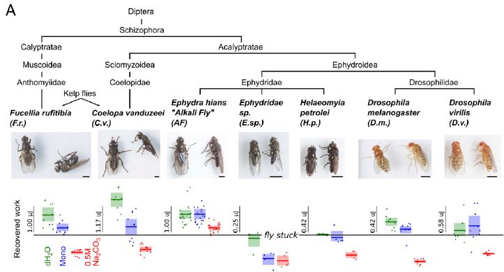
There is a lot here; we'll focus on just a few key points. Don't get bogged down with the complexity of the figure.

The graphs at the bottom show the work done when a fly exits a particular fluid. To illustrate, look at the first data set (at the left). The green data is for water. Skip the blue data for the moment. The red data is for 0.5 M Na₂CO₃. What matters is that one set of data is positive (above the x-axis), whereas the other set is negative (below the x-axis). That is, these flies will "pop out" of water, but not out of the sodium carbonate solution.

That data set is for the fly Fucellia rufitibia. The parts of the graph to the right show similar data for other flies. The general pattern is about the same for all cases -- except one. For the third fly (from the left), the data show that it will pop out of both the water and the sodium carbonate solution. That fly is Ephydra hians, known as the alkali fly, as you can see from the labeling above the graph.

Back to the blue data. It is labeled Mono (and elsewhere in the article as MLW); that's Mono Lake water. Mono Lake is a lake in the California mountains, noted for its alkalinity. It is about pH 10: not as alkaline as that sodium carbonate solution, but quite alkaline for biology. The Mono results vary for the various flies, usually somewhere in between the water and sodium carbonate results. For the alkali fly, Mono is as good as water. That is, these flies can pop out of Mono just as if it were pure water. And they can still pop out of the sodium carbonate solution, which is even more alkaline.

The data on the graphs is quantitative, and is given in microjoules (µJ). However, the scale is different for each fly. The main point is to compare the data for a particular fly under the three conditions. You can do that qualitatively by visual inspection.

The upper parts of the graph show the flies, and a chart of how they are related.

This is Figure 3A from the article.

So flies can pop out of water, and one kind can even pop out of sodium carbonate solution. How did they get into the water? In the work above, the experimenters put them under water. But getting wet is a concern for flies, and being hydrophobic is a useful trait.

The alkali fly studied here is from Mono Lake. It lives around the lake, and goes into the alkaline water to lay its eggs -- and to feed. It emerges looking essentially dry -- as Mark Twain observed a century and a half ago. The current work provides lab data showing that this fly is unusual in how it responds to sodium carbonate -- and it really is the specific salt, not just the alkalinity, that matters. It is superhydrophobic. (The work here is on a fly from Mono Lake, but similar alkali flies are found around the world.)

What makes the flies so hydrophobic? Dense hairs on the body, and lots of wax. As a result, the flies are surrounded by an air bubble when they enter the water; the air bubble protects them, and also serves as an oxygen source. No new principles there, but these flies do it to the extreme.

News story: Scuba diving flies use bubbles to feed underwater. (M Andrei, ZME Science, November 21, 2017.) For those who don't get to the article, this page includes the Mark Twain story and part of the quotation.

The article: Superhydrophobic diving flies (Ephydra hians) and the hypersaline waters of Mono Lake. (F van Breugel & M H Dickinson, PNAS 114:13483, December 19, 2017.) Check Google Scholar for a freely available copy from the authors. The article is from Caltech.

More about superhydrophobic materials...
* Disease transmission by sneezing -- in wheat (July 29, 2019).
* Water droplets on a trampoline (April 9, 2016).

More from Mono Lake:
* NASA: Life with arsenic (December 7, 2010).
* Arsenic and photosynthesis (September 9, 2008).

Posts about unusual flies include...
* Progress toward an artificial fly (December 6, 2013).
* TIGER discovers smallest known fly; does it live in the head of tiny ants? (July 31, 2012).

There have been no previous Musings posts invoking Mark Twain. However, a Twain book -- a science book (sort of) -- is listed on my page Books: Suggestions for general science reading: Mark Twain, 3,000 Years Among the Microbes (1905).

Influence of the food additive trehalose on Clostridium difficile?

February 23, 2018

Clostridium difficile (C dif) is a bacterium that can cause serious intestinal problems. A recent article makes a connection between C dif and the sugar trehalose, which is increasingly being used as a food additive.

The first finding... Some important, highly virulent strains of C dif are able to use trehalose efficiently as a food source. The following figure makes this point...

The figure shows how various strains of C dif grow on various carbon sources.

The strains of C dif are shown at the bottom of each part of the graph. They include two specific types of strains, called RT027 and RT078. The first set of data points includes ten "other" strains.

The y-axis is a measure of the growth of the C dif strains under the specified conditions.

The left-hand data set is for growth on DMM. That is a minimal medium, with no carbon source. Bacteria should not grow on this medium. And they don't. You can take the value shown for the DMM case to mean "no growth".

The middle data set is for growth on glucose. That is the minimal DMM with glucose added. All the strains grow, as expected.

The right-hand data set is for growth on trehalose. You can see that the two new types of strains grow on trehalose, but the "other" strains do not.

The concentrations of the two sugars used here are equivalent, on the basis of mass or energy content. Trehalose is a disaccharide. The level of sugar used here is quite low; that is the point: this is about the ability to use low levels of trehalose efficiently.

This is Figure 1 from the article.

The results above show that two important lines of C dif have acquired the ability to grow on a low level of trehalose.

The authors suspect that the high virulence of these strains is somehow related to the recent increase in use of trehalose as a food additive. However, we stress that the result above, per se, says nothing about the importance of the sugar to the bug's pathology.

The following experiment explores the role of trehalose in a C dif model infection...

In this experiment, mice were infected with a strain of the RT027-type of C dif, a strain that can use trehalose. The curves show survival of the infected mice (y-axis) vs time (x-axis). Two conditions: the mice were or were not fed trehalose.

The results show that adding trehalose (lower line on the graph; dashed) reduced the survival of the infected mice. About twice as many of the infected mice died when trehalose was included in the diet (compared to no trehalose).

The mice used here had a humanized microbiome.

This is Figure 3b from the article.

We have shown two pieces of evidence relating trehalose to C dif. One shows that some highly virulent strains of C dif can grow on trehalose. The other shows that trehalose increases the severity of infection with such a strain in a mouse model.

The article provides more experiments, which fit with the general picture. The bottom line is not entirely clear; there is no direct evidence that dietary trehalose affects humans infected with C dif. However, the article certainly raises the possibility.

While this is being investigated further, it is reasonable to suggest that those who have a C dif infection minimize consumption of trehalose, as a precaution. Further, institutions with large numbers of older people, those most at risk for serious C dif infections, might avoid serving trehalose.

Trehalose is a natural sugar. Most humans can metabolize it, though it is probably not commonly a major component of our diet. It is generally considered safe. For an introduction to this sugar, see Wikipedia: Trehalose. That page notes the new article discussed here.

News stories:
* Food Additive May Be Worsening Clostridium Difficile Epidemic. (A Berezow, American Council on Science and Health (ACSH), January 4, 2018.)
* Dietary sugar linked to bacterial epidemics. (D Pathak, Baylor College of Medicine, January 4, 2018. Now archived.)
* Expert reaction to study looking at dietary trehalose (a sugar additive) and virulence of clostridium difficile infection in a mouse model. (Science Media Centre, January 3, 2018.)

* News story accompanying the article: Microbiology: Pathogens boosted by food additive. (J D Ballard, Nature 553:285, January 18, 2018.)
* The article: Dietary trehalose enhances virulence of epidemic Clostridium difficile. (J Collins et al, Nature 553:291, January 18, 2018.)

Previous post about C dif: Fecal transplantation as a treatment for Clostridium difficile: progress towards a biochemical explanation (February 8, 2015).

Previous posts that mention trehalose: none.

Another example of natural sugars that may be more important for their effect on our microbiome than on their direct nutritional content: Breastfeeding and obesity: the HMO and microbiome connections? (November 14, 2015).

My page Organic/Biochemistry Internet resources has a section on Carbohydrates. It includes a list of related Musings posts.

February 21, 2018

CRISPR: Making specific base changes -- at the RNA level

February 20, 2018

CRISPR is often described as a tool for editing genes. However, in its familiar form, CRISPR most commonly inactivates genes. A Cas enzyme is guided by a piece of RNA to a specific site in a gene, where it cuts the gene. Subsequent repair of the cut leads to inactivation of the gene. There have been numerous technical developments to work out practical applications of the original CRISPR approach as well as variations.

A recent article on CRISPR has two novel features that we have not discussed in previous Musings posts. First, it targets RNA rather than DNA. Second, it makes a specific base change in the RNA, rather than cutting it.

We'll illustrate the new system with a specific example from the article...

Part A (left) describes the system. Part B (right) shows some results.

The header for Part A gives some background information. The work here involves a mutant gene with a disease-causing mutation from G to A at site 878. That mutation changes codon 293, which should code for tryptophan, to a stop (termination) codon.

The goal is to edit that particular A back to a G. In fact, what is actually done is to edit it to an I (inosine); I and G are equivalent in this context. That is, a codon with I is translated just as if the I were a G.

Part of the messenger RNA sequence is shown. Several A bases are numbered. One of them is colored; that is A-46, the mutant A.

Below the mRNA are three guide RNAs. Look at the first of those. It has a hairpin at the left end. The rest of it is almost entirely paired with the mRNA; pairing is shown by a vertical line between guide and message. The one exception is for that A-46. The guide RNA has a C at that position, giving an A-C mispair. That mispair targets the editing event.

The other two guide RNAs are almost the same. The only difference is that the region of pairing with the mRNA is moved slightly to the right. But the basic plan -- including the specific mispair for targeting -- is the same.

The results are shown in two ways in Part B.

The graph shows that each of the three guides resulted in about 20-40% editing at the desired site. One of them appears to be significantly better. Positioning of the guide matters.

The bar labeled NT is for a negative-control guide RNA, which is non-targeting (NT). It leads to a low, but not zero, level of editing.

The heat map shows the same results, but also shows a little more. It also shows the editing that was observed at any of the other A sites -- off-target sites. It's hard to tell from the figure, but there is a low level of editing at A-40 using the first guide.

This is from Figure 4 of the article.

Overall, the results above show that Cas-mediated RNA editing -- to make a specific base change -- works at a significant level. Getting 20-40% editing would restore useful protein levels in many cases. The results also show that details matter, and that we must be alert for off-target effects.

Comments...

How do we get Cas to act on RNA? This is a different Cas: Cas13 (rather than the more common Cas9). Cas13 acts naturally on RNA.

How do we edit a base? The editing here uses a variant of a natural enzyme, called adenosine deaminase. That enzyme removes the amino group from base A to make base I (which, as noted, behaves just like base G for many purposes).

The enzyme is abbreviated ADAR, which stands for adenosine deaminase acting on RNA.

That is, the editor here is built from known parts. The Cas13 protein targets RNA, but has been modified here so that it does not cut it. The adenosine deaminase has been modified to partner with the Cas13 protein and its guide RNA. (Development continues... The scientists have already improved the editing enzyme to reduce off-target changes.)

Why do we want a system to edit RNA rather than DNA? One answer is that we want both; we want more tools so we have more choices. But an advantage of editing RNA is that it may be more flexible. An edit to DNA is presumably permanent; any ill effects are permanent, too. Messenger RNAs and their resulting proteins are typically shorter-lived. Repeated treatment may well be necessary, but that also means that the treatment can be tuned over time. That is probably a good tradeoff, especially for new and profound tools such as gene editing.

The work here adds more tools to the gene-editing toolbox.

News stories:
* RNA Editing Possible with CRISPR-Cas13. (R Williams, The Scientist, October 25, 2017.)
* Researchers engineer CRISPR to edit single RNA letters in human cells. (Broad Institute, October 25, 2017.) From the lead institution.

* News story previewing the article (in an earlier issue of the journal): 'Base editors' open new way to fix mutations. (J Cohen, Science 358:432, October 27, 2017.) Also discusses a recent article that reports doing a similar specific base edit in DNA.
* News story accompanying the article: Molecular biology: Enhancing the RNA engineering toolkit. (L Yang & L-L Chen, Science 358:996, November 24, 2017.)
* The article: RNA editing with CRISPR-Cas13. (D B T Cox et al, Science 358:1019, November 24, 2017.)

More base editing... Treating progeria by editing the gene (March 23, 2021).

Previous CRISPR post: Laika, the first de-PERVed pig (October 22, 2017).

Next: CRISPR connections: p53? cancer? (October 6, 2018).

A post with a complete list of Musings posts on various gene-editing tools, including CRISPR, TALENs and ZFNs... CRISPR: an overview (February 15, 2015).

Low temperature treatment for auto exhaust?

February 18, 2018

A recent trend in automotive engineering is that engines are releasing exhaust at lower temperatures (T) than they used to. More efficient use of the fuel means that less heat is wasted. And that is creating a new problem: the catalytic converters that remove pollutants from the exhaust require high T to function properly.

There is now an official goal of achieving emissions standards at exhaust T of 150° C. That is about 100 degrees lower than before.

A recent article reports progress in developing a catalyst that will oxidize carbon monoxide, CO, in the exhaust at 150° C.

Here are some results...

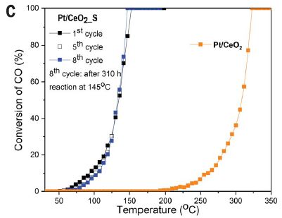
The graph shows how two catalysts deal with CO as a function of T.

For simplicity, let's say that the y-axis is a measure of the rate of oxidation of CO.

You can see that one curve, to the right (orange symbols), shows that the catalyst becomes effective between 200-300 °C.

The other set of results, to the left (black, blue symbols), shows that this catalyst becomes effective between 50-150 °C. There are multiple curves here. The catalyst was tested after various amounts of use. It didn't matter much; the catalyst gave about the same results each time it was tested.

The y-axis is not a simple measure of rate. The scientists are using a flow cell system; that, of course, mimics a real auto exhaust treatment system. T is ramped up during the test. It is not clear in the article exactly how they calculate the y-axis parameter that is shown. I do think it is intended to be effectively a rate measurement.

This is Figure 1C from the article.

Taken at face value, the results above show that the new catalyst, at the left, is effective at about 150 degrees lower T than the old one. In particular, it is very effective at the new target T of 150 °C. Further, it is reasonably effective even during a cold start.

What are these catalysts? The labels say Pt/CeO₂ (old catalyst; right) and Pt/CeO₂_S (new catalyst; left). Pt/CeO₂ means they are based on cerium oxide, with Pt atoms on the surface. And that "_S"? It means that the catalyst was steam-treated before use: 750 °C, several hours. This "hydrothermal aging", as they call it, changes the nature of the surface and allows it to operate at lower T.

As usual for catalyst development, what the scientists did here was largely empirical. They tried various ways of making catalysts to see what works. They have only limited information about how the improvement actually works, but it seems that the steam pre-treatment stabilizes the position of the Pt atoms on the cerium oxide surface. (Similar treatment of other potential catalysts leads to various results, sometimes making them worse.)

The catalyst works at a lower T, but it also retains its activity when exposed to high T. That's important, too; sometimes, with high loads, engines operate very hot.

News story: New catalyst meets challenge of cleaning exhaust from modern engines. (Phys.org, December 14, 2017.)

The article: Activation of surface lattice oxygen in single-atom Pt/CeO₂ for low-temperature CO oxidation. (L Nie et al, Science 358:1419, December 15, 2017.)

Posts about catalysts and catalyst development include...
* A better catalytic sponge: degrading plastics, and more (August 11, 2020)
* Breaking C-F bonds? (October 26, 2018).
* Making hydrocarbons -- with an enzyme that uses light energy (November 17, 2017).
* Photocatalytic paints: do they, on balance, reduce air pollution? (September 17, 2017).
* 2 + 2 = 4: Chemists finally figure it out (October 9, 2015).
* A simpler way to make styrene (July 10, 2015). Links to more.

More cerium oxide: A Christmas present: Using concentrated sunlight to split water and CO₂ (February 18, 2011).

A post about vehicle emissions: What's the connection: ships and lightning? (October 14, 2017).

Added February 13, 2024. This post is listed on my page Introductory Chemistry Internet resources in the section Lanthanoids and actinoids.

What's wrong with the flu vaccine?

February 16, 2018

Warning...Confusion ahead. This is about the flu vaccine -- and why it doesn't work very well.

You've probably heard that the vaccine doesn't work very well. You've probably heard it during the current flu season. And last flu season. Maybe each flu season -- back to about 2005.

So, the flu vaccine effectiveness (VE) dropped starting in 2005? No, it's just that was the first year anyone actually measured it. It's not a trivial matter to measure it. It's not even trivial to decide what the term means. Somehow, it should reflect effectiveness out in the real world, not just a lab measurement.

A new article reports a systematic analysis of the flu vaccine in Canada during the 2015-6 season. The big message is that the VE wasn't very good.

The details don't matter much, and some of the findings may not be well accepted. However, here is an example of the findings, so you have a sense of what people are dealing with...

The vaccine contained two main components. The VE for them turned out to be about 43% and 54%. For one of them, there was a good match between the vaccine virus and the virus that actually circulated in Canada that year. For the other, there was not a good match. The one with the good match gave the 43% VE. Now, the two VE numbers may not be significantly different, but still... don't we expect the matched vaccine to do better? Anyway, neither VE is good.

The big conclusion is that there is more to flu VE than antigenic match. The article explores other factors -- with no clear conclusions. If you read further into this work, be prepared for lots of numbers, sometimes interesting numbers, and plenty of confusion.

What to do? There are two major areas of work to improve the flu vaccine. One is to develop a universal flu vaccine -- at least one that is effective against a wide range of strains. Currently we have the annual ritual of guessing what strain to use for the vaccine, and then hoping the match is good. Sometimes it is, sometimes not; as the current work indicates, even a match does not guarantee success.

Universal -- or broad-range -- flu vaccines are in the works. Will they really work? We'll see -- eventually. There is no guarantee that a universal vaccine will solve the problems. However, it would at least allow focus on a single vaccine.

The other major area of work is to move from making flu vaccines in eggs to cell culture. Again, this is undoubtedly a good idea, but it -- alone -- may or may not affect VE.

Developing effective control of influenza remains a challenge.

A reminder... Musings does not give medical advice. This post is not intended to influence a person's choice of what to do with the flu vaccine.

It is important that scientists are analyzing the vaccine, and trying to figure out what its weaknesses are. Understanding its weaknesses is, one might expect, a key to developing better flu vaccines. Thus we focus here on the negatives because that is central to developing better vaccines. But it is a different issue than whether a person should take the current vaccine -- or not.

News story: Study identifies factors that may lower flu vaccine protection. (L Schnirring, CIDRAP, October 6, 2017.) Good overview of the work, including its uncertainties.

* Commentary accompanying the article; it may be freely available: Beyond Antigenic Match: Moving Toward Greater Understanding of Influenza Vaccine Effectiveness. (E Belongia, Journal of Infectious Diseases 216:1477, December 19, 2017.)
* The article, which is freely available: Beyond antigenic match: possible agent-host and immuno-epidemiological influences on influenza vaccine effectiveness during the 2015-16 season in Canada. (D M Skowronski et al, Journal of Infectious Diseases 216:1487, December 19, 2017.)

The day before I posted this item, the US CDC published their current estimates of the VE in the US for this flu season. I have not had time to read the article carefully, but the bottom line is clear enough... It's not very good. The article, which is freely available: Interim Estimates of 2017-18 Seasonal Influenza Vaccine Effectiveness -- United States, February 2018. (B Flannery et al, MMWR 67:180, February 16, 2018.) Those with a serious interest in the flu vaccine issue may well find the article worth reading. (E Belongia, listed above as author of the commentary, is a co-author of this article. There are no Canadian institutions listed for author affiliations.)

* * * * *

A recent post about flu vaccine problems: The nasal spray flu vaccine: it works in the UK (April 12, 2017). (From the title, it may not seem to be a problem. However... )

More: Using antibodies from llamas as the basis for a universal flu vaccine? (December 7, 2018).

Posts on flu and flu vaccines are listed on the supplementary page Musings: Influenza (Swine flu).

February 14, 2018

An eye that forms an image using a mirror

February 13, 2018

The human eye has a lens, which focuses the incoming light onto the retina, where the actual light receptors are.

There is another way to focus light -- with a mirror. Is it possible that Nature discovered this, too?

A recent article provides a rather detailed analysis of the eye of the scallop Pecten maximus. This unusual eye has intrigued biologists for centuries; one reference in the article is from 1795. But only in recent decades have biologists come to understand that a mirror is a key part of the scallop eye -- and that a few other animals, invertebrate and vertebrate, also have mirrors in their eyes.

Here are some pictures. They are at increasing magnification; see the scale bars.

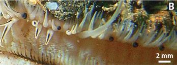
	A photograph showing five of the eyes. There be as many as 200 eyes on such an animal.
Having trouble finding them? One is directly above the "2 mm" label, lower right. A small dark circle. The others are in a line towards the left. This is Figure 1B from the article.

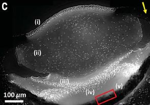
A cross-section of an eye, showing the major structures... (i) cornea, (ii) lens, (iii) distal retina, (iv) proximal retina, (v) concave mirror.

Yes, that seems to be a rather long parts list; we'll come back to this later.

The image is taken with fluorescence microscopy, with the nuclei labeled. The dots are cell nuclei. You can see that the lens area has few cells, and that the retinas are rich in cells.

This is Figure 1C from the article. The yellow arrow (upper right) is the direction of incoming light. The red rectangle marks the region studied further.

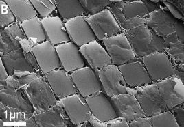
The mirror, as seen from the top by scanning electron microscopy.

The squares are crystals of guanine (the base known from nucleic acids).

The mirror is not just a plane of guanine crystals. The crystals are stacked, in a regular spacing. It is the ordered alternation of different materials, guanine crystals and cellular fluids, that makes the mirror.

Those squares really are squares. The authors state, in the figure legend: "The crystals are 1.23 × 1.23 ± 0.08 µm (N = 20) with internal corner angles of 90.16 ± 2.78 ° (N = 28) (means ± SD)."

It must be quite a feat of biosynthesis to make these mirrors!

Some of them don't look so good. I suspect that there was considerable damage during preparation for electron microscopy, and that the authors chose good crystals to measure.

This is Figure 2B from the article.

What about the properties of these mirrors? Some results...

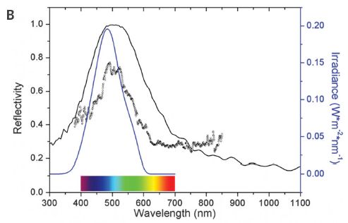
The graph shows three things, each plotted against the wavelength of light (x-axis).

Start with the worst-looking curve... the rather jagged black dashed curve. It shows the reflectivity of the mirror, as measured in the lab. The reflectivity is shown on the left-hand y-axis scale. The curve shows a peak near 500 nm.

The blue curve shows the spectrum of light that the animal would typically receive (at a depth of 20 meters). For this curve, use the right-hand y-axis scale. The important observation is that the reflectivity response of the eye-mirror is similar to the spectrum of available light.

Finally, the solid black curve near the top. That is a curve the scientists have calculated for the reflectivity of the mirror. It's similar to the actual, measured curve. This suggests that the scientists have a reasonable understanding of the mirror's properties.

This is slightly modified from Figure 3B from the article. (I removed an inset from the figure.)

We started by noting that the scallop eye uses a mirror to form an image. Then, we found that it actually contains a lens, too. The authors note that the lens is not very good. That would seem to lead to many questions, but the general answer for now is that we have no idea why this animal developed this optical system.

The picture of the eye structure, above, also shows there are two retinas. The work in the article suggests that the mirror can focus light onto both of them. It may be that the two retinas are used for different parts of the field of view.

Overall, the article presents a fascinating analysis, at multiple levels, of an unusual eye. Those interested in biology, chemistry, physics, or astronomy may enjoy browsing the article or even pursuing this topic further.

News stories:
* Understanding How Scallops View the World. (Inside Science (American Institute of Physics), November 30, 2017.)
* Scallops Have Eyes, and Each One Builds a Beautiful Living Mirror. (E Yong, Atlantic, November 30, 2017.)
* The Scallop Sees With Space-Age Eyes - Hundreds of Them. (C Zimmer, New York Times, November 30, 2017.)

The article: The image-forming mirror in the eye of the scallop. (B A Palmer et al, Science 358:1172, December 1, 2017.)

Other posts on the diversity of animal eyes include...
* A see-shell story (February 21, 2016).
* Where are the eyes? (August 19, 2011).
* How many eyes does it have? (March 12, 2010).

And even one about a non-animal... Is the warnowiid ocelloid really an eye? (October 12, 2015).

For more mirrors... Could we block seismic waves from earthquakes? (June 23, 2014).

Squares are not common in biology, but another example is included on my page Unusual microbes: Square bacteria.

When did mammals take on daylight?

February 11, 2018

The dominant large animals are now the mammals. But until about 66 million years ago the dinosaurs played that role.

Mammals were around back then, they just weren't dominant. They were small, often underground -- and nocturnal. Being nocturnal presumably helped them avoid getting eaten by the big ones.

We need some terms, to describe when an animal is active. Unfortunately, a couple of the terms are not common, so ...
- Nocturnal: active mainly at night.
- Cathemeral: no particular daily rhythm; may be active day or night.
- Diurnal: Active mainly during daytime.

In the modern world, we are diurnal, as are many of our common mammals. What happened? There has long been a hypothesis that mammals emerged to dominance after the dinosaurs left -- making it safe. (More specifically, it was the non-avian dinosaurs that left.) It could well be that mammals also began to explore daytime on the same time scale.

Evidence? Not much. It's hard to tell whether a fossil animal was nocturnal or diurnal; skeletal features are not a reliable indicator of day-use preferences.

A recent article provides some evidence on the matter. Look at the following graph...

The graph shows the number of lineages of mammals with various life styles over time.

The life styles are the three we listed above.

The x-axis scale is shown at the top; the scale is in Ma -- millions of years ago. Of particular interest is the vertical red-dashed line, labeled K-Pg, at about 65 Ma. That is the Cretaceous-Palaeogene mass extinction event.

The pattern is clear: Before the K-Pg line, all mammals were nocturnal. Cathemeral mammals began to appear at about the time of the dinosaur extinction, with diurnal mammals to follow.

The blue and green regions of the time scale are for the Jurassic and Cretaceous periods, respectively.

This is Figure 3b from the article.

What is the basis of the graph? We have already noted that fossils are not reliably informative on the issue. What the scientists did here was to collect information about the day-use preferences of 2,415 modern mammals. They then made a phylogenetic analysis, focusing on the character at hand. It leads to a best estimate of when new day-use traits developed in mammalian lineages.

The graph shows a correlation. It does not -- cannot -- show causality. In fact, a second analysis in the article, with somewhat different assumptions, shows the emergence of cathemeral mammals slightly before the dinosaur extinction. In that case, it is still plausible that the dinosaur extinction allowed for a major expansion of mammals using daylight. In any case, the article is an interesting exploration of mammal history, with a focus on how we use the day.

News story: Mammals switched to daytime activity after dinosaur extinction. (Phys.org, November 6, 2017.)

The article: Temporal niche expansion in mammals from a nocturnal ancestor after dinosaur extinction. (R Maor et al, Nature Ecology & Evolution 1:1889, December 2017.) Check Google Scholar for a freely available copy. What's available there includes a preprint at BioRxiv.

A post about a nocturnal monkey: Monogamy (January 30, 2013).

Most recent post on dinosaur extinction: How the birds survived the extinction of the other dinosaurs, why birds don't have teeth, and how those two points are related (July 30, 2016). Links to more.

Is Mars wetter than Earth -- underground?

February 9, 2018

The headline was Martian water stored underground. And the following graph was prominent...

The y-axis is the water content of the rocks, and the two curves are clearly labeled Earth and Mars.

The Mars curve is always higher. The Mars rocks always have more water.

The x-axis is depth below the planetary surface. This is underground water.

This is Figure 1 from the news story in Nature (by Usui).

That's what got my attention. Mars' water is underground. Or at least, it would be if this were real data.

Following up -- checking out the article behind the headline and news story... It's not quite as exciting as we might have hoped, but it is interesting.

First, some background... Mars is generally thought to be low on water. However, why it is dry is quite unclear. It should have started with about the same percentage of water as Earth. It's certainly plausible that a lot of water has evaporated from the lightweight Mars or got swept away by solar winds, but the best estimates of such losses really suggest there should still be plenty around. If so, where is it?

Sub-surface ice is one possibility. The new article provides another. The authors did computer modeling of Earth and Mars crustal rocks. The conclusion is that the Martian rocks are, relatively speaking, sponges. They hold more water than Earth rocks. The difference increases with depth, which corresponds to higher pressure.

What's the difference between Earth and Mars rocks that leads to their different water-binding? That's complicated, but it is based on at least some evidence. The basalt rocks on Mars are more highly oxidized. And the temperature profile with depth leads to hydrated minerals sinking, thus helping to ensure that water is sequestered underground.

The amount of water the modeling predicts is substantial. The authors estimate that underground hydrated rocks could account for the entire estimated water content of Mars.

How robust are the conclusions? It's hard to tell. There are a lot of assumptions. What the article does is to show that, at least with certain reasonable assumptions, it is plausible that Mars could have a lot of underground water, in the form of hydrated rocks.

So, the graph above is for computer water -- theoretical water. Maybe we should send someone up there and dig a hole.

News stories:
* Study: Martian Surface Water Was Absorbed by Planet's Crust. (Sci.news, December 24, 2017.)
* Water on Mars absorbed like a sponge, new research suggests. (Phys.org, December 20, 2017.)

* News story accompanying the article: Planetary science: Martian water stored underground. (T Usui, Nature 552:339, December 21, 2017.)
* The article: The divergent fates of primitive hydrospheric water on Earth and Mars. (J Wade et al, Nature 552:391, December 21, 2017.)

More about water on Mars:
* Water on Mars? InSight finds none (September 19, 2022).
* A lake on Mars? (August 24, 2018).

Posts that may be -- but probably aren't -- about water on Mars:
* What causes gullies on Mars? (September 8, 2014).
* Water at the Martian surface? (August 27, 2011). A recent follow-up article, by the authors of the article discussed in this post, makes the water interpretation of the work less likely.

Among other posts about or referring to Mars...
* Nanopore sequencing of DNA: How is it doing? (November 13, 2017).
* Perchlorate on Mars surface, irradiated by UV, is toxic (July 21, 2017).

February 7, 2018

The origin of SARS: getting closer

February 6, 2018

Briefly noted...

Considerable evidence has been accumulating to implicate bats as a major reservoir of coronaviruses. However, the specific origin of any specific virus, such as the SARS virus, is not clear.

A recent article provides more evidence, and perhaps brings us closer to the origin of SARS.

The article involves extensive surveillance, over several years, of a particular cave. Many coronaviruses were isolated and sequenced. The big finding is that the collection of coronaviruses in the cave includes all of the key gene sequences found in the SARS virus.

The scientists did not find the SARS virus itself in the cave. However, one can easily imagine it arising by recombination between the viruses that were found there.

The article does not show that this cave is the source of the SARS virus. There may be other sites that contain the necessary viral genes. Perhaps some other cave already contains the SARS virus itself. The scientists have not demonstrated that the suspect recombination actually occurs, or that the virus can get from this cave to the human populations. What the article does is to provide more support for simple plausible scenarios for what might have happened. We no longer need to hypothesize that all the SARS sequences were near to each other in a somewhat restricted environment. We now know of one specific example.

Could it happen again? Could another "SARS" arise in a bat cave and cause problems in humans? The authors suggest that continuing surveillance would be prudent.

News stories:
* Bat cave study sheds new light on origin of SARS virus -- Newly discovered SARS strains in bats hold genetic clues to the evolution of a human pandemic strain. (EurekAlert!, November 30, 2017.)
* Scientists Close in on Origin of SARS. (Chinese Academy of Sciences, December 8, 2017.)

The article, which is freely available: Discovery of a rich gene pool of bat SARS-related coronaviruses provides new insights into the origin of SARS coronavirus. (B Hu et al, PLoS Pathogens 13:e1006698, November 30, 2017.)

A recent post broadly about coronaviruses: Bats and the coronavirus reservoirs (July 25, 2017).

A post about the early history of another coronavirus: When did the SARS-2 (COVID-19) virus arise? A window into how a zoonosis starts (June 22, 2021).

There is more about SARS and coronaviruses on my page Biotechnology in the News (BITN) -- Other topics in the section SARS, MERS (coronaviruses). It includes links to good sources of information and news, as well as to related Musings posts.

Stone age human violence: the Thames Beater

February 5, 2018

Can you break someone's head open by beating them over the head with a club?

When did humankind discover the answer to that question?

Would the club shown in the following picture do the trick?

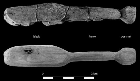
This is Figure 2 from a recent article. We'll explain it a little more below.

Well, there is one way to find out.

Some results...

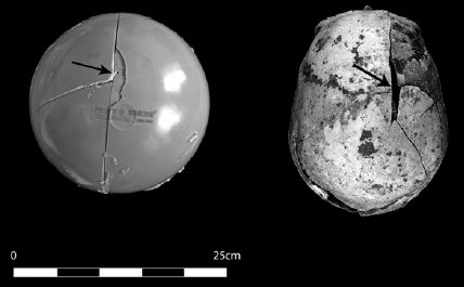
It worked.

This is Figure 8 from the article. The scale bar is for the left-hand item only.

Let's fill in some of the details...

In the first figure, the top item is an actual wooden club, known as the Thames Beater. It is considered Neolithic, about five thousand years old. The bottom item is a replica, used in the current work. It was made to match the original as closely as possible, including using the same kind of wood.

The actual test was done with a model for the human skull. The model is designed to recreate the response to injury. In the second figure above (Fig 8) the left-hand item shows the model after having been hit with the replica club. The right-hand item is an old skull from an archeological site. The nature of the damage is similar in both cases. The pattern of damage is consistent with high-impact trauma, rather than a fall or crushing.

There is much one can wonder about here, as to how closely the scientists have in fact made revenant replicas of the club and the skull. Presumably, the test system will be critiqued and developed.

Taken at face value, the work provides evidence that Neolithic man could break skulls. And that he wanted to.

News stories:
* Morbid Experiment Proves This Neolithic Weapon Was an Effective Skull Crusher. (G Dvorsky, Gizmodo, December 14, 2017.)
* Experiments show Neolithic Thames beater could be used to kill a person. (B Yirka, Phys.org, December 12, 2017.)

The article: Understanding blunt force trauma and violence in Neolithic Europe: the first experiments using a skin-skull-brain model and the Thames Beater. (M Dyer & L Fibiger, Antiquity 91:1515, December 2017.)

From the abstract: "The difficulty in identifying acts of intentional injury in the past has limited the extent to which archaeologists have been able to discuss the nature of interpersonal violence in prehistory. Experimental replication of cranial trauma has proved particularly problematic due to the lack of test analogues that are sufficiently comparable to the human skull."

* * * * *

A recent post on human violence: In the aftermath of gun violence... (January 8, 2018). Links to more.

A recent post with more about what ancient man could do: The oldest known dog leash? (January 23, 2018).

More about skull injuries:
* Head injuries in Neandertals: comparison with "modern" humans of the same era (February 22, 2019).
* Skull surgery: Inca-style (August 21, 2018).

More about trauma: Type O blood and survival after severe trauma? (July 7, 2018).

More wood: Artificial wood (November 3, 2018).

Role of neoantigens in surviving pancreatic cancer?

February 4, 2018

More survival curves. This time for pancreatic cancer, a cancer with notoriously poor prognosis. They are from a recent article, which offers a clue as to why some people survive pancreatic cancer longer than others.

For each graph in the following figure, a population of people with pancreatic cancer is divided into two parts of approximately equal size. The survival curves for those two sub-populations are then compared.

A quick inspection...

In one part, the survival curves for the two sub-populations are about the same.

In the other case, they are not. And that's the point.

This is the right-hand side of Figure 2b from the article.

What's this about? It is about cancer immunology. And that means it is hard to explain.

The upper graph is labeled neoantigen quality. The lower graph is labeled neoantigen quantity. You can see, then, that it is quality that matters.

Neoantigens? This is about the tumor antigens: those found on the surface of the tumor. The term neoantigens means that they are new antigens -- ones not found normally.

Let's step back...

The role of the immune system in fighting cancer has become a hot field. Recent developments of immunotherapy are allowing people with advanced cancers to be cured. However, only a small percentage of the patients treated show much response. In a recent post, we noted that cancers with a high mutation rate are more susceptible to immunotherapy [link at the end].

It is known that the tumors of those who survive longer with pancreatic cancer are more infiltrated with T cells. This is evidence of a greater immune response. The question is, why do some people have more of an immune response?

That leads to the current work... The scientists looked at the antigens -- the neoantigens -- on the tumors. Cataloging tumor antigens is complicated, but that is what they did. Beyond that, they developed a model to rank the antigens by "quality": how well each antigen works in promoting an effective immune response. For now, let's accept that they did these things, and not worry about how.

What the figure above shows is that, whatever it is they did, it is of some value. Simply counting the antigens wasn't informative. Comparing survival of people with more neoantigens to survival of those with fewer showed no difference (lower graph). However, quality of antigens was informative. Comparing survival of people with "higher quality" antigens to survival of those with lower quality antigens showed a difference (upper graph).

And what do they mean by high quality antigens? There is no easy answer. The work involves looking at multiple characteristics, including similarity to known pathogen antigens and known binding affinities in the immune system. It also involves a lot of modeling and fitting. The work should not be taken as a definitive presentation of antigen quality, but rather as an indication that it is an important idea, and may be accessible

The conclusion? People will survive pancreatic cancer longer if their tumor makes more good new antigens. That enhances the ability of the immune system to fight the cancer.

What's the significance of the finding? Most importantly, it would seem to represent a step forward in our understanding of cancer. The ability to predict antigen quality probably will improve. But what do we do with the information? We'll see. As we have already noted, cancer immunology is becoming a hot field, but one still full of mysteries.

News story: New Study Findings Unlock the Secret of Why Some People with Pancreatic Cancer Live Longer than Others. (Memorial Sloan Kettering Cancer Center, November 8, 2017.) From the lead institution. Now archived.

* News story accompanying the article: Cancer immunotherapy: How T cells spot tumour cells. (S Sarkizova & N Hacohen, Nature 551:444, November 23, 2017.) This item accompanies two articles. One is the article discussed here. The other is more broadly about cancer immunotherapy; it also deals with predicting antigen quality.
* The article: Identification of unique neoantigen qualities in long-term survivors of pancreatic cancer. (V P Balachandran et al, Nature 551:512, November 23, 2017.)

Background post on cancer immunotherapy: Predicting who will respond to cancer immunotherapy: role of high mutation rate? (October 6, 2017).

More pancreatic cancer: Pancreatic cancer: another trick for immune evasion (August 1, 2020).

Previous pancreas post: Making a functional mouse pancreas in a rat (February 17, 2017).

My page for Biotechnology in the News (BITN) -- Other topics includes a section on Cancer. It includes an extensive list of relevant Musings posts.

A mutation, found in a human population, that extends the human lifespan

February 2, 2018

Here are two survival curves, from a recent article...

You can see that the blue curve is shifted to a longer lifespan, compared to the red curve. (The mean is shifted by about 7 years; the median is shifted by 10 years.)

The red curve is labeled +/+; the blue curve is +/-. That is, the red curve is for wild types; the blue is for heterozygotes -- those who carry one copy of a mutation.

What organism? Humans.

Individuals who died prior to age 45 were not considered in this analysis, as you can see from the x-axis above.

This is slightly modified from Figure 2 of the article. I added the genotype symbols for the curves.

What is this mutation? It is in a gene called SERPINE1, which codes for a protein called plasminogen activator inhibitor-1 (PAI-1). The particular mutation studied here is a null mutation, leading to total loss of active protein. SERPINE1 is known to affect senescence; work in lab mice has shown that those with a mutant copy of SERPINE1 have various metabolic improvements -- and live longer. The graph above extends this to humans. Other results reported in the article show other metabolic improvements, consistent with what was expected from the mouse work.

For example, the frequency of diabetes was 7% in the wild types (8 out of 127), and zero (0/43) in the heterozygotes.

How did we get a test of this gene in humans? The results are for a natural population, a small community that is reproductively isolated. Genealogical analysis identified a particular couple that introduced the mutation into the community six generations ago.

It is an intriguing finding. Taken at face value, we have a single mutation that affects human lifespan by several years. That lifespan change is accompanied by metabolic changes that are considered good. Further, the effects are supported by work in the mouse model system; that means that we have at least some understanding of how the mutation works.

The SERPINE1 gene protein, PAI-1, is important. People in the population with two copies of the mutant gene have significant bleeding and heart problems; they clearly have too little PAI-1. The current work may suggest that we normally have too much of it. But why? The heterozygotes have half the normal (homozygote) level of PAI-1. If that is better as judged by lifespan and some metabolic studies, why do we normally have twice as much? Why isn't the gene regulated to produce a lower level of PAI-1, if that would be better? Are we missing something more in the story -- something important?

Would it be beneficial to try to inhibit SERPINE1 with a drug? Would drug development based on the mouse model be useful? If anti-aging drugs are tested in humans, how long would it take to become convinced they are helpful? And safe? In fact, work with such a drug is in progress.

News stories:
* Rare Gene Mutation Linked to Longer Lifespan in Amish. (Sci.news, November 17, 2017.)
* Why these Amish live longer and healthier: An internal 'Fountain of Youth'. (Science Daily, November 15, 2017.) Includes a discussion of the early history of studying the mutation in the community, and also a discussion of the drug work.

The article, which is freely available: A null mutation in SERPINE1 protects against biological aging in humans. (S S Khan et al, Science Advances 3:eaao1617, November 15, 2017.)

A recent post on senescence: A treatment for senescence? (June 4, 2017).

Another example of looking at isolated populations for gene effects: Cataloging gene knockouts in humans (July 10, 2017).

My page for Biotechnology in the News (BITN) -- Other topics includes a section on Aging. It includes a list of related Musings posts.

More about bleeding: Type O blood and survival after severe trauma? (July 7, 2018).

January 31, 2018

Wind energy: effect of climate change?

January 30, 2018

Use of wind energy is increasing. Wind energy is a renewable energy source, not using fossil fuels. Increased use of wind energy is one good response to the threat of global warming.

But we might ask... Will climate change affect the availability of wind energy? After all, wind is an aspect of climate.

A new article addresses the question. The conclusions are not very clear, but the article is worthy of note just for addressing the question.

Here is the general plan... Take a particular proposed scenario for overall climate change. Calculate predictions for wind, using various climate models.

Of course, there are various possible climate scenarios; what happens will depend much on how we reduce C emissions. And there currently are multiple climate models that can be used to predict the winds. We also note that useful wind energy depends in a complex way on wind speed.

The following figure shows a sampling of the predictions...

The graphs show predicted change in available wind energy, as a percentage, vs time over this century.

Each graph is for one geographical region. These four are for parts of the Americas, north to south as you go across the figure.

The results shown here are all for one particular climate scenario.

The various curves on each graph are for different climate models -- ten of them.

The big picture...
* The predictions are very different for different regions.
* There is sometimes major disagreement between the models for a particular region.

Looking at some specifics... The models generally predict that, under this climate scenario, wind energy availability in the Mexico area will be fairly stable. In the eastern Brazil area, it may increase substantially over this century. In the two US areas, it may decrease substantially. All of those statements are generalities, with substantial uncertainty because of the different predictions from the different models.

This is part of Figure 4a from the article. The rest of Fig 4a contains 12 more such graphs, for other regions around the world. I chose the ones above just as a sampling -- conveniently the top row of the figure.

What do we get out of all of this?
- First, the results show that there may be changes -- large changes -- in the availability of wind energy as climate change proceeds. There even seems to be a general pattern... As climate change progresses, there will be, broadly, less wind in the northern hemisphere and more in the southern hemisphere.
- Second, our ability to predict those changes is limited at this point. A striking example is the one model for Central US that makes a very different prediction from all the other models. Scientists can ask why the model does this. What feature of this model, compared to the others, leads to the big difference? Then, can we resolve which model -- which feature -- is "correct"?

Overall, the article is a caution that wind energy may not be easily predictable over the long term.

Comment... Climate change is a highly politicized issue. Science gets caught in the political debate, and both sides use it poorly at times. There are things that science understands well about climate change -- and things it does not. When people on one side exaggerate how much science does or does not know, it encourages the other side to do likewise. That doesn't help!

News stories:
* As The Climate Warms, Wind Power Could Shift Southward. (P Patel, Anthropocene, December 14, 2017.)
* UK wind power potential could fall by 10% by 2100 because of climate change. (Carbon Brief, December 11, 2017.) Includes the complete Fig 4a (even the complete Figure 4) from the article, if you want to see the predictions for the other regions. It also includes a discussion of the reasons behind the north-south wind shift.
* Expert reaction to research on the impact of global warming on wind energy in the northern hemisphere. (Science Media Centre, December 11, 2017.) As usual, this source presents comments from several people in the field. Unusually, the several comments here are in general agreement... An interesting study, the conclusions of which are questionable. Again, that is not so much a criticism as a plea that more is needed in a difficult area. But we should specifically note... All of the commenters are from the UK, and they tend to emphasize the UK. In fact, the effects predicted for the UK are quite small compared to the predictions for most other regions.

The article: Southward shift of the global wind energy resource under high carbon dioxide emissions. (K B Karnauskas, Nature Geoscience 11:38, January 2018.)

Musings has had little to say about wind energy, but wind is the subject of several posts. Here are a couple; each links to more.
* Atmospheric rivers and wind (May 9, 2017).
* Improved high altitude weather monitoring (July 18, 2016).

I have listed this post on my page Internet Resources for Organic and Biochemistry under Energy resources. It includes a list of some related Musings posts.

Lightning and nuclear reactions?

January 28, 2018

One recent morning, as I worked on a draft of this post, the weather forecast offered a chance of thunderstorms for the afternoon. Had they occurred, there might have been an increase in the amount of the carbon isotope C-13 in the atmosphere. So says a recent article.

We all know that lightning involves energy. A lot of energy. But did you know... that energy can cause nuclear reactions in the atmosphere?

Here's the idea...

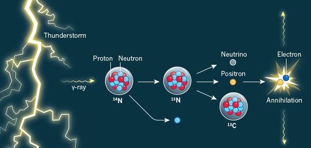
The figure starts with a lightning bolt. Among other things, it can lead to gamma (γ) rays.

If a γ-ray of appropriate energy strikes the nucleus of an ordinary nitrogen atom in the atmosphere, it can lead to the ejection of a neutron. The original N-14 nucleus is converted to the lighter isotope N-13. The ejected neutron is shown, as a light blue dot, just below the new N-13 nucleus. (Nuclear symbols can be written in the form ¹⁴N or N-14. The former is more formal; the latter is easier to type, and I will usually use it.)

N-13 is an unstable nucleus. Half life 10 minutes. It soon emits a positron. That leaves a C-13 nucleus, which is stable.

The positron (β⁺) is antimatter; it soon encounters its matter counterpart, the ordinary electron (β^-). They annihilate, with the production of a pair of γ-rays. Those γ-rays are shown at the right, though not labeled there. What's particularly important is that the γ-rays from the annihilation have a distinctive energy -- the energy that corresponds to the mass of the particles.

This is Figure 1 from the news story by Babich in Nature. The figure is also in the Science Alert news story.

What's above is theory. We might expect those things to happen.

What's new is that scientists have now detected the distinctive γ-rays from the positron-electron annihilation during a thunderstorm. Look...

The figure shows an energy spectrum of the γ-rays for a particular event during a thunderstorm.

The y-axis is a measure of the γ-rays; the x-axis shows their energy.

There is a clear peak at about 0.5 megaelectronvolt (MeV). The predicted value for the positron-electron annihilation is 0.511 MeV.

The analysis is considerably more complex than the graph might suggest. The graph here is for a time period already determined to be a time of increased γ-rays, and suspected of being due to annihilation.

This is Figure 4a from the article.

Those results provide evidence for what is shown in the figure above: nuclear reactions, releasing antimatter positrons, during thunderstorms.

News stories:
* Breaking: Thunderstorms Observed Triggering Nuclear Reactions in The Sky -- They what now? (P Dockrill, Science Alert, November 22, 2017.)
* Storms Generate Thunder, Lightning and ... Antimatter? (C Choi, Discover (blog), November 22, 2017.)

* News story accompanying the article: Atmospheric science: Thunderous nuclear reactions. (L Babich, Nature 551:443, November 23, 2017.)
* The article: Photonuclear reactions triggered by lightning discharge. (T Enoto et al, Nature 551:481, November 23, 2017.)

Recent post about lightning: What's the connection: ships and lightning? (October 14, 2017).

Recent post about positrons, and also dealing with the distinctive γ-rays upon positron-electron annihilation: The major source of positrons (antimatter) in our galaxy? (August 13, 2017).

More about thunderstorms: High-voltage thunderstorms: how high? (April 29, 2019).

More about C-13: Life on Earth 4.1 billion years ago? (November 2, 2015). The amount of C-13 in a material is used to help identify its origins. The current work might make one wonder whether the production of C-13 during thunderstorms could upset our usual interpretations of what C-13 levels mean. The amount of C-13 made during storms, while interesting, is probably negligible, and not likely to affect our usual interpretations of C-13. However, this is just one of the possible reactions; there is a possibility that C-14 production during thunderstorms might be comparable to that from the usual sources.

Also see: Would weather forecasting be improved by considering the isotopes in atmospheric moisture? (May 2, 2021).

Can prions, which cause brain disease, be transmitted by skin?

January 26, 2018

Prion diseases are degenerative brain diseases caused by a misfolded protein. That misfolded protein, called a prion, can cause other copies of the protein to misfold, thus promoting the agent. The most common human prion disease is Creutzfeldt-Jakob disease (CJD); a variant form is related to bovine spongiform encephalopathy (BSE; mad cow disease).

Prion diseases are dependent on the host having a copy of the gene for the protein; the prions are not autonomous. However, they can be transmitted, usually with low efficiency, in some cases. The transmission of BSE to humans by eating beef, resulting in vCJD, is well documented, but inefficient. Prions can also be transmitted by medical procedures; for example, brain material that happens to contain prions might be put into the brain of another person. Medical practice now recognizes this possibility, and there is little current transmission of prions by such procedures.

What about skin? Is it possible that prions could be transmitted via the skin? Could a brain disease be transmitted by skin tissue?

Look at the following figure...

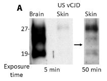
There are three lanes of data, each with results for the prion protein in a patient with vCJD. The first lane (left) is for brain tissue, the second (center) is for skin tissue. You can see a strong response in the brain lane, and a very weak response in the skin lane. Weak but positive.

To reinforce the observation for the skin lane, the sample was incubated longer: 50 minutes instead of 5 min (see times at the bottom). That makes the skin result clearer. Weak but positive.

The test here is a Western blot. Protein samples are run on a gel, and then tested with an antibody that binds to the desired protein.

The antibodies are labeled with radioactivity; that is what is detected here. The times shown at the bottom are time of exposure of the film.

The messy result seen in the first lane is typical of prion preparations.

This is Figure 1A from the article.

The result above shows that, for one particular vCJD patient, there is a low level of prion protein in the skin tissue.

Follow-up work showed that a low level of prion was found in all 23 CJD patients (sporadic or variant) tested. This work included using a more sensitive assay, one that detects in vitro function of the prion protein. As a control, 15 people without prion disease were tested; none had any detectable prion protein in the skin samples.

The question we asked at the start was whether the skin could be a source for transmission. The evidence above merely shows prion protein that can be detected by lab assays. Is it in a form that is transmissible? A good test would be to try to infect an animal with the material from the skin. Here are some results...

Survival curves. Mice were injected with skin samples from three people.

The green line across the top shows the results for mice that received skin samples from a healthy human donor. All the mice survived.

The other two curves are for mice that received skin samples from people with CJD. All these mice died.

This is Figure 4A from the article.

Overall, the article shows that people with CJD have a low level of infectious prion in their skin.

What are the implications? There is no suggestion that people with CJD transmit the disease by ordinary contact, such as shaking hands. However, there is reason for some concern about handling any tissue from people -- or presumably other animals -- with prion diseases. Reasonable precautions are in order.

An intriguing question is... Might the finding allow for a simpler method of diagnosis of prion diseases?

News stories:
* Researchers find infectious prions in Creutzfeldt-Jakob disease patient skin. (Medical Xpress, November 22, 2017.)
* Infectious Prions Detected in Skin of Patients With Neurodegenerative Creutzfeldt-Jakob Disease. (MedicalResearch.com, November 23, 2017.) Interview with a senior author.

The article: Prion seeding activity and infectivity in skin samples from patients with sporadic Creutzfeldt-Jakob disease. (C D Orrú et al, Science Translational Medicine 9:eaam7785, November 22, 2017.)

A previous post about tissue specificity of prions: Prion diseases -- a new concern? (March 19, 2012).

Next prion post: Mineral licks and prion transmission? (May 8, 2018).

For more about prions, see my page Biotechnology in the News (BITN) - Prions (BSE, CJD, etc). It includes a list of related Musings posts. Some of these deal with the possibility that Alzheimer's disease is something like a prion disease, and may be transmissible.

January 24, 2018

The oldest known dog leash?

January 23, 2018

Here is the data...

This is part of Figure 4 from the article.

The figure shows a person and several dogs. The person has a bow and arrow; he is presumably a hunter.

Importantly, two of the dogs appear attached to the hunter. The connections would seem to be leashes.

The picture above is a cave painting, from Saudi Arabia. (It is a tracing of the original. The full figure in the article also includes a photograph of the actual art.) It is thought to be about 8000 years old.

There is considerable uncertainty about the date, as usual for cave paintings. Perhaps there is uncertainty about interpreting the picture.

Why is this of interest, beyond being a nice picture? Uncertainties aside, let's assume those really are dogs on leashes, part of a hunting scene a few thousand years ago. The cave painting then provides evidence for one stage of the story of dog and man. That is, it is a document with historical information -- about the history of dog domestication.

The figure above shows more than just leashes. There are numerous dogs, all peacefully around the hunter, and looking in the same direction.

That figure is one of 147 paintings, from two sites, that seem to show dogs as part of a hunting scene. Several include leashes.

Is it possible that the art is fictional? Sure, but it presumably builds on the real world. Would an artist have invented the scene shown above without some knowledge of dogs involved in hunting?

News stories:
* Wall carvings in Saudi Arabia appear to offer earliest depiction of dogs. (B Yirka, Phys.org, November 21, 2017.)
* 8,000 years old rock art in Saudi Arabia documents the earliest known use of dog leashes. (A Micu, ZME Science, November 21, 2017.)

The article: Pre-Neolithic evidence for dog-assisted hunting strategies in Arabia. (M Guagnin et al, Journal of Anthropological Archaeology 49:225, March 2018.)

Previous post that involved a leash: The opah: a big comical fish with a warm heart (July 13, 2015).

Among other ancient art...
* Images from 30,000-year-old motion pictures (July 22, 2012).
* Leopard horses (December 2, 2011).

There is more about art on my page Internet resources: Miscellaneous in the section Art & Music. It includes a list of related Musings posts.

More old things from Saudi Arabia: The oldest known plants (November 2, 2010).

More about dog domestication:
* The oldest known sick dog? (March 14, 2018).
* It's a dog-eat-starch world (April 23, 2013).

Previous post on dogs: Predicting success in training guide dogs -- role of good mothering (November 27, 2017).

More domestication: Domestication of the almond (August 26, 2019).

More about what ancient man could do: Stone age human violence: the Thames Beater (February 5, 2018).

Gene therapy and stem cells: A child gets new skin

January 22, 2018

A simple story... A child has a genetic disease that destroys his skin. He now has normal skin. The treatment? Take skin cells from the child, add to them a normal copy of the gene that is defective, grow new skin, and transplant it to the child. It worked.

Of course, there is much detail, and much uncertainty, but it does seem an important development.

Here is a diagram of what happened...

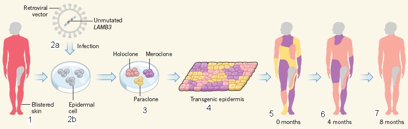
Start with the diagrams of the child at the sides. At the left (part 1 of the figure) is what he looked like before the treatment. You can take the red color in this drawing as meaningful; he (substantially) lacked normal skin. At the extreme right (part 7), 8 months into the treatment, he has normal skin.

The child has junctional epidermolysis bullosa (JEB). It is due to a mutation in a gene for laminin. The mutation prevents the skin layers from staying attached properly; the result is extreme blistering and, effectively, loss of skin. That's not just a cosmetic issue; the skin is a primary defense against pathogens. JEB is a serious disease, often fatal.

The scientists constructed a retroviral vector that contained a normal copy of the laminin gene (part 2a, at the top). They isolated skin (epidermal) cells from the child, and infected them with the new vector (part 2b).

The cell preparation at this point contained cells at various stages of development, or "stemness". These are shown in part 3 with various colors, to help you follow them (and with some names, which may not be so helpful).

The cell mix was grown in the lab into a skin layer (specifically the epidermis layer; part 4). It is a mixture of the various cell types, as you can see from the colors.

The lab-grown genetically-corrected skin was transplanted to the child. The resulting skin was analyzed at various times (parts 5, 6, 7). By 8 months, the child had normal skin over 98% of his body. The amounts from the various original cell types varied. The main trend was an increasing fraction of cells derived from the original "holoclone" cells; these are the cells that are most fundamentally stem cells -- capable of proliferating. That is, the new skin was ultimately derived from the stem cells in the transplant.

This is slightly modified from Figure 1 from the news story, by Aragona & Blanpain, in Nature. I added numbers for the individual parts, for ease of referring to them.

Figure 1 of the article itself includes photographs of the child "before" and "after".

At the time of the treatment, the child was considered in critical condition. The treatment was done as a last resort. Although all of the steps are logical, there had been only limited experience putting it all together to treat skin loss by transplantation of genetically modified skin. The current case is far more severe than any treated this way previously, with multiple operations to transplant skin to about 80% of the child's body.

It's now two years since the treatment began, and the child continues to do well. He is going to school, playing football (soccer), and generally living a normal life -- of course with plenty of monitoring.

What are the uncertainties? They fall into two classes. First, we do not know the long term outcome for this child. Second, we do not know the generality of the treatment. Nevertheless, this seems to be a very exciting development -- for this child, and who knows for how many more.

News stories:
* Extraordinary epidermis regeneration in child via combo stem cell-gene therapy. (The Niche (blog from a stem cell lab), November 8, 2017.)
* 'Extraordinary' tale: Stem cells heal a young boy's lethal skin disease. (M Blau, STAT, November 8, 2017.)
* Boy is given new skin thanks to gene therapy. (Science Daily, November 8, 2017.)

* News story accompanying the article: Gene therapy: Transgenic stem cells replace skin. (M Aragona & C Blanpain, Nature 551:306, November 16, 2017.)
* The article: Regeneration of the entire human epidermis using transgenic stem cells. (T Hirsch et al, Nature 551:327, November 16, 2017.)

An earlier post reporting a bold pioneering step in dealing with a very sick child: Genome sequencing to diagnose child with mystery syndrome (April 5, 2010).

Another post involving a genetic condition affecting skin: Why some people don't leave fingerprints (September 19, 2011).

More about making new skin: A handheld printer that can print cells onto a severe burn (February 16, 2020).

See my Biotechnology in the News (BITN) pages for Cloning and stem cells and for Agricultural biotechnology (GM foods) and Gene therapy. Each contains an extensive list of related Musings posts. It is interesting how the two topics have come together.

How to "dye" carbon fiber -- with titanium dioxide

January 20, 2018

Carbon fiber is a useful material, with excellent mechanical properties and chemical inertness. And it is black.

The inability to dye carbon fiber almost follows from its chemical inertness. It's hard to get anything to stick.

A recent article reports making carbon fibers any color you want, by putting a white powder on the surface.

Here is an example...

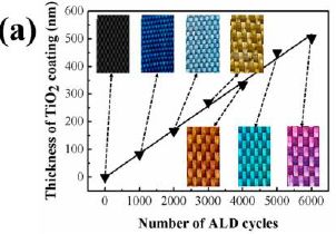
	Start with the pretty pictures. They are pieces of woven carbon-fiber fabric that have been colored, using the new treatment. The first picture (upper left) shows the original, untreated fabric. The others show pieces of fabric after various amounts of treatment. What is that treatment? Addition of a surface layer of titanium dioxide, TiO₂, by atomic layer deposition (ALD).
The graph x-axis shows the number of cycles of ALD. The y-axis shows the thickness of the resulting TiO₂ layer. The thickness depends linearly on the amount of treatment; it is about 0.1 nm per cycle. The pictures then show the resulting fabric colors. This is Figure 3a from the article.

The color here is "structural color", a term used to indicate color by a process distinct from the common absorption of light. It is due to reflection at the thin TiO₂ layer. The thickness of that layer is on the order of the wavelength of the light, leading to complex reflection, including interference patterns. Exactly how the light reflects depends on the thickness of the film; that's the basis of the effect seen above.

You might wonder why the TiO₂ sticks. The authors note the concern and offer some hypotheses, but really aren't sure. It may have to do with the small TiO₂ interacting with occasional reactive groups on the fiber surface. However it gets started, as the process continues, TiO₂ is binding to the previous layer of TiO₂.

The colored fabrics can be washed repeatedly (ordinary home laundering), with only little loss of color. Further, the colored fabrics have only slightly reduced mechanical properties.

Although the process is not fully understood, it may be a step toward being able to make carbon fiber materials colored as you wish.

News story: Carbon fibre gets a colourful makeover. (E Stoye, Chemistry World, October 13, 2017.)

The article: Facile and Effective Coloration of Dye-Inert Carbon Fiber Fabrics with Tunable Colors and Excellent Laundering Durability. (F Chen et al, ACS Nano 11:10330, October 24, 2017.)

A recent post about structural color: Coloring with graphene: making a warning system for structural cracks? (June 2, 2017).

Also see:
* Added May 4, 2023. Paint without pigment (May 4, 2023).
* Why do many tarantulas have blue hair? (March 7, 2016).

More about dyeing fabrics: A better way to make (the dye for) blue jeans, using bacteria? (March 5, 2018).

A recent post about TiO₂: A "greener" way to make acrylonitrile? (January 6, 2018). Carbon fiber was also noted in this post.

Monkey malaria in humans?

January 19, 2018

If we are going to keep track of diseases, and try to reduce them, it would help if we really knew what caused them.

A recent article illustrates the problem. It shows that an outbreak of malaria was not caused by the usual suspects, but by a distinct pathogen: a monkey malaria parasite, Plasmodium simium.

The common human malaria pathogens are P falciparum and P vivax. About twenty other malaria parasites are known for primates, eight of which are known to be able to infect humans. P knowlesi, whose primary host is macaque monkeys, causes considerable human malaria in Southeast Asia. Except for that, it is thought that most human malaria is transmitted (by mosquitoes) from other humans. Transmission of malaria from non-humans to humans -- so-called zoonotic transmission -- is considered uncommon.

What now? The short version of the story is that (human) malaria recently reappeared in a region of Brazil from which it had been eliminated. It appeared to be vivax malaria. However, the new work shows that it was actually simium malaria, which is known to be in the area. Why the confusion? The two parasites are hard to tell apart -- except by using modern molecular techniques. In the new work, the scientists used sequencing of the mitochondrial genome.

Does it matter? Well, it may not matter to those who got sick. But it does matter to those who want to understand disease transmission. In this case, the two diseases are transmitted differently. One is transmitted between humans, whereas the other is transmitted from monkeys to humans. (In both cases, transmission is by a mosquito vector.)

As you read this story... What really matters is the source of the infection. It matters whether the disease is being transmitted only from humans or from monkeys. It isn't the name of the bug that matters, but the transmission pattern.

If the new malaria is indeed monkey malaria from the reservoir in the forest, it means that the disease had never really been eliminated from the region. It was merely held in check. The re-emergence may well be due to changing patterns of forest use, including for tourism.

Disease is complicated.

News story: Malaria parasite spreads from howler monkeys to humans. (S Boseley, Guardian, September 1, 2017.)

* "Comment" article accompanying the article. Freely available: Plasmodium simium: a Brazilian focus of anthropozoonotic vivax malaria? (M J Grigg & G Snounou, Lancet Global Health 5:e961, October 2017.)
* The article, which is freely available: Outbreak of human malaria caused by Plasmodium simium in the Atlantic Forest in Rio de Janeiro: a molecular epidemiological investigation. (P Brasil et al, Lancet Global Health 5:e1038, October 2017.)

You will encounter the word autochthonous in this story, especially in the article itself. It means native. In context, an autochthonous case is one that has not been imported (say by someone who had been in a region with malaria). Therefore, there must be a local (native) source.

There is apparently some uncertainty whether the vivax and simium are really distinct species, or just different strains; it doesn't matter.

* * * * *

A recent post on malaria: Malaria and bone loss (September 10, 2017).

A recent post exploring other zoonoses -- diseases transmitted to humans from other animals: Bats and the coronavirus reservoirs (July 25, 2017). Also check the linked item there on "One health".

There is a section of my page Biotechnology in the News (BITN) -- Other topics on Malaria. It includes a list of Musings posts on malaria, and on mosquitoes in general.

January 17, 2018

A new species of orangutan?

January 16, 2018

There are three species of orangutans, not two, according to a new article.

It's not that the scientists found a new animal, but that they examined the knowns more carefully, and concluded that one population is sufficiently distinct that it deserves species status.

Pongo tapanuliensis, the Tapanuli orangutan.

Tapanuli refers to three districts in Sumatra (such as South Tapanuli).

This is trimmed and reduced from a figure in the Mongabay news story.

Determining species is not easy. The common separation of orangutans into two species, Bornean and Sumatran, was established only in 2001. It required genome analysis to make the distinction clear.

In the new work, a team of scientists reports that one population of orangutans in Sumatra is morphologically and genetically distinct from the other orangutan species.

The work began with a single specimen of a dead animal. Features of the head, including the teeth, seemed quite distinct from what is considered normal for Sumatran orangutans. Genetic analyses, including animals from all three groups, confirmed the differences, and suggested that the new species split off from the others about 3.4 million years ago (mya). For comparison, the split between the other two orangutan species is dated at only 0.7 million years ago.

There is very limited data behind the proposal to designate a new species here. The article makes the case, but it needs confirmation, probably including more data, and discussion. The population of the proposed new species is only about 800 individuals, in a limited area -- as best they understand it now. Whether the species designation holds up or not, the work is a call for further investigation of the Sumatran orangs. The Tapanuli orangutans are at least an endangered population; they may be an endangered species.

If you are struck by the hair of the animal shown above... The authors note that the hair of this species is "frizzier" than for the others. (I doubt that any orangs use combs.)

News stories:
* Anthropologists describe third orangutan species. (Phys.org, November 2, 2017.)
* The Eighth Great Ape: New orangutan species discovered in Sumatra. (M Erickson-Davis, Mongabay, November 2, 2017.) Eight great ape species? That refers to living species. Three orangs, as discussed here; two gorilla species; chimps; bonobos; humans.

The article: Morphometric, Behavioral, and Genomic Evidence for a New Orangutan Species. (A Nater et al, Current Biology 27:3487, November 20, 2017.)

More orangs... Re-introducing captive animals into the wild: an orang-utan mix-up (June 27, 2016).

More apes... Do apes say "hello"? (September 14, 2021).

More from Sumatra... Does the moon affect earthquakes? (October 21, 2016).

More about dividing things up among species: An interesting skull, and a re-think of ancient human variation (November 12, 2013).

How long does a supernova event last?

January 14, 2018

A nova is a new object appearing in the sky. A supernova is an unusually bright nova. It is now understood that supernovae are due to stars exploding as they die. As one might expect in some general sense for an explosion, a supernova rapidly becomes much brighter; it then decays.

Here are some supernova data, from a recent article...

That's a complex figure, but we can summarize it and get the main message.

The figure shows data for the brightness of two supernova events over time. The data for one event are shown by the big colored points over the top part of the graph. The data for the other event are shown by the dashed lines at the lower left.

The big picture... The brightness for one event (iPTF14hls; top) remained high over at least the first 400 days shown here. It declined slowly after that. The brightness for the other event (SN1999em; lower left) declined dramatically over about 100-150 days.

SN1999em is a typical supernova of this type. In fact, it was thought that such supernova events could not last more than about 150 days. And that's the point: the event shown across the top lasted far longer. iPTF14hls is an unusual supernova event.

A new article presents this recent unusual supernova event. The data for SN1999em are shown for comparison.

Don't try to compare the brightness of one supernova with the other here. They are plotted on different scales -- though this is not very clear in the article. Since the spacing of magnitude units is the same on both scales, we can compare the rates of decline; that's what we want here.

And yes, the bigger the magnitude number, the less bright the object is.

The big gap at around 300 days? The object was behind the Sun during that time.

The various colors for the data are for different spectral bands. The various symbols are for different observing stations.

This is slightly modified from Figure 1 of the article. I added the label identifying the supernova for the top data set. Also, I removed some stuff at the top of the full figure that I did not want to get into.

Not only is the new event extended, but there seem to be increases in brightness along the way. For example, there is a substantial increase in brightness at about 100 days, and there is a small peak at about 200 days.

It's probably not hard to look at the new data and suggest that this is a more complex event, with multiple explosions along the way. It is as if the star is exploding one piece at a time. That's fine, but astronomers have not seen such a complex supernova event before. Further, the authors are unable to provide any simple explanation in terms of current understanding of how stars collapse and explode.

Interestingly, there is evidence that this star may have exploded a little about 60 years ago, though one cannot connect the earlier event to the current one with certainty. "Exploded a little"? That's an interesting idea in itself.

The new supernova may be an example of a pulsational pair-instability supernova. But what that really means -- what really happened here -- is not at all clear. It is something new, something that cannot be explained at this point. It is truly a scientific discovery.

News stories:
* Zombie star' cheats death again and again, dumbfounding scientists. (T Puiu, ZME Science, November 9, 2017.)
* Supernova Discovery Challenges Theories of How Certain Stars End Their Lives. (Sci.News, November 9, 2017.)

* News story accompanying the article: Astronomy: The star that would not die. (S Woosley, Nature 551:173, November 9, 2017.)
* The article: Energetic eruptions leading to a peculiar hydrogen-rich explosion of a massive star. (I Arcavi et al, Nature 551:210, November 9, 2017.)

More supernovae...
* The major source of positrons (antimatter) in our galaxy? (August 13, 2017).
* Could you find debris from a supernova in your backyard? (April 27, 2016).

Pumping tin

January 12, 2018

You know how to pump water? You could pump tin the same way, right? Well, you would have to melt it first. And that creates a new problem: the pump must be able to operate at high temperature.

The melting point of tin is actually fairly low, only 232 °C. However, being able to pump it at much higher temperature (T) could facilitate its use in heat transfer systems. That is actually the big motivation behind the current work, besides simply demonstrating a high-T pump. In a new article, scientists develop a pump that can operate at over 1200 °C. Maybe even at 1400 °C.

Here is the plan for the pump...

Most of the figure is a diagram of the pump. In general, it looks fairly normal at this level.

At the lower left is a photo of part of the pump in action. The color is due to the heat. That's the main point of showing the figure. (The color in the upper part, which is a diagram, is artistry.)

This is trimmed from Figure 1 of the article. (I have removed one part of the figure, at upper right. The two lines going up from the gears go to the part I cut out.)

The secret to operating a pump at such a high T? The materials, of course. Ceramics. Graphite. The chemical inertness of such materials at high T is known, but ceramics can be brittle. What is novel is making a functioning pump out of them.

How well did the pump survive? The following figure shows the gears after 72 hours of operation...

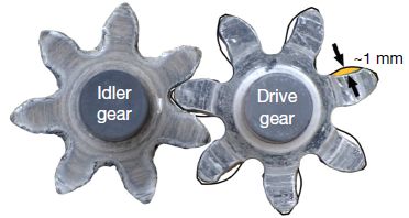
Look at the gear on the right. The black line shows the original shape. You can see that there is significant wear.

This is Figure 5 from the article.

It works, but needs improvement.

The authors note plans for such improvement. For example, they note that the gear material used here was chosen partly for convenience for initial testing; better materials are available.

The article claims that this is the highest temperature at which pumping has been demonstrated. It shows that ceramics can be used to make a high-T pump; the scientists plan work to make it practical. They even envision going on to pump silicon. The melting point is 1420 °C, and they would hope to pump it at over 2000 °C. Pumping molten tin or silicon could be a good way to transfer energy.

Video: Pumping Liquid Metal (Tin) at 1200C (~2200F). (YouTube, 2 minutes.) Interesting, but not well labeled. Background music, but no useful narration. Some of it is too fast to follow at a single viewing.

News stories:
* Pumping liquid metal at 1,400 °C opens the door for better solar thermal systems -- A ceramic pump can handle the heat; careful engineering prevents it from cracking. (M Geuss, Ars Technica, October 13, 2017.)
* Ceramic pump moves molten metal at a record 1,400 degrees Celsius. (Phys.org, October 11, 2017.)

* News story accompanying the article: Engineering: Liquid metal pumped at a record temperature. (K Lambrinou, Nature 550:194, October 12, 2017.)
* The article: Pumping liquid metal at high temperatures up to 1,673 kelvin. (C Amy et al, Nature 550:199, October 12, 2017.)

Posts about pumping include...
* Lamb-in-a-bag (July 14, 2017).
* pH and the color of petunias (March 26, 2014).
* Caltech engineer turns rat into jellyfish (September 22, 2012).

More about tin... A step toward a practical thermoelectric converter: get the oxide out (October 11, 2021).

January 10, 2018

A look at Chopin's heart

January 9, 2018

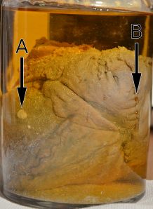
That's it.

It's in a jar of a brown fluid, which is probably cognac.

This is the Figure from the article.

Frederic Chopin died in 1849. His heart was removed from his body, according to his wishes. It was put in a bottle, as shown above, and given to his sister. The heart is now at a church in Warsaw, and is examined from time to time.

Chopin was only 39 when he died, and the cause of his death has never been clear.

A new article reports briefly on the most recent examination of Chopin's heart, in 2014 -- 69 years after the previous examination.

Among the prominent findings are three lesions near arrow A in the figure. The authors note that these are most likely from tuberculosis.

Arrow B points to stitching to the left ventricle, following its opening during the autopsy.

There is more, but not much more. It's a two-page article, with observations and some interpretation -- and much uncertainty. Heart specialists may enjoy the detail. But the big story here is the big picture: the preservation and examination 165 years later of Chopin's heart.

News stories, both of which provide good overviews:
* Chopin's Preserved Heart May Offer Clues About His Death -- Scientists who recently examined the organ have suggested that Chopin died of complications from tuberculosis. (B Katz, Smithsonian, November 9, 2017.)
* Examination of Chopin's pickled heart solves riddle of his early death -- Scientists diagnose rare complication of tuberculosis following analysis of heart stored in jar of cognac for 170 years. (R McKie, Guardian, November 4, 2017.) Overstates the conclusions, but still, a useful story.

The article: A Closer Look at Frederic Chopin's Cause of Death. (M Witt et al, American Journal of Medicine 131:211, February 2018.)

Previous heart post: Heart regeneration? Role of MNDCMs (November 10, 2017).

Another examination of an old specimen for possible TB... A new approach for testing a Llullaillaco mummy for lung infection (August 17, 2012).

More TB: A new vaccine against tuberculosis? (November 9, 2018).

There is more about music on my page Internet resources: Miscellaneous in the section Art & Music. It includes a list of related Musings posts.

In the aftermath of gun violence...

January 8, 2018

Guns are a political issue in the United States.

In December 2012 a gunman went into the Sandy Hook Elementary School in the US state of Connecticut and killed 20 children (and six adults). Such a mass killing, especially of children, provokes debate about gun laws -- a least for a while.

A new scientific article reports some data about guns, in the context of the Sandy Hook incident.

The question the authors examined is... What is the effect of a major shooting, which becomes a major news event, on subsequent gun events?

The following figure summarizes some of the main findings...

The graph plots data for two gun-related phenomena over time. One is shown as blue bars; the other is shown as a black line.

A quick inspection of the graph shows that both phenomena reached a peak in early 2013 -- immediately after the Sandy Hook event.

What are these two phenomena? The graph labels them well. The black line shows sales of guns in the US (left-hand y-axis). The blue bars show accidental gun-related deaths of children (right-hand y-axis). (The death data is given as deaths per 100,000 population per month.)

In both cases, the data is shown in a way that emphasizes the variation from "average". Zero is the average value over the time period. There is nothing of particular interest except for the peak values already mentioned. The magnitudes of the values at that peak were the largest magnitudes found, whether positive or negative.

This is Figure 2 from the article.

That is, the Sandy Hook event, with its news coverage, was quickly followed by a burst of gun sales and accidental gun-deaths of children.

The data above for accidental deaths of children is given as a rate, and compared to the average. We can add that the blue bar for that peak period represents 18 deaths above the average -- an increase in the absolute death rate of about 60%. (There were also 39 extra deaths of adults. The overall increase in the gun-death rate was about 20%.) Note that these numbers are all for accidental deaths from guns, not criminal activity.

The graph shows a correlation; it does not show there is a causal connection. However, if we assume, for the moment, a causal connection... It may be good to note that most people who responded to Sandy Hook had no direct connection with the original event itself. The results shown above are national data. Most who responded -- if indeed the data shown are a "response" -- knew of the story only through the news media, including the political discussion.

I will just leave it at that: an example of collecting evidence about the effect of guns. There is no claim that we understand what is behind the data shown here, or that this is the complete story. And it is not for me to get into the political issues.

News stories:
* Sandy Hook shooting aftermath: Increased gun sales, more accidental deaths by firearms. (EurekAlert!, December 7, 2017.) Includes some general discussion of gun issues, including the importance -- and difficulty -- of collecting data.
* After a Mass Shooting, a Surge in Accidental Deaths -- Research on the Sandy Hook massacre shows public focus on firearms after a massacre leads to more tragedy, particularly among children. (P Mosendz, Bloomberg, December 7, 2017.) An example of coverage by the general news media.
* Sandy Hook mass shooting triggers weapons purchase. (K Jaramillo, LatinAmerican Post, December 17, 2017. Now archived.) A view from outside the US.
* Wellesley Faculty Find that a Jump in Gun Sales and Accidental Gun Deaths Followed the 2012 Sandy Hook Shootings. (Wellesley College, December 8, 2017.) From the lead institution -- a two-hour drive from Sandy Hook. Links to several news stories in the mainstream general media.

* "Policy forum" accompanying the article: Gun-violence research: Saving lives by regulating guns: Evidence for policy. (P J Cook & J J Donohue, Science 358:1259, December 8, 2017.) This is a broader discussion of gun violence and gun laws. The emphasis is on right-to-carry laws. There is only minimal discussion of the current article,
* The article: Firearms and accidental deaths: Evidence from the aftermath of the Sandy Hook school shooting. (P B Levine & R McKnight, Science 358:1324, December 8, 2017.)

More about human violence...
* Stone age human violence: the Thames Beater (February 5, 2018).
* Violence within the species -- in various mammals; implications for the nature of humans (December 6, 2016).
* Human violence (November 28, 2011).

The previous mention of a gun was in the post What happens when a lithium ion battery overheats? (February 19, 2016). It was a heat gun in this case.

A "greener" way to make acrylonitrile?

January 6, 2018

Acrylonitrile, for use in making polymers and carbon fiber, is made from petroleum. A new article offers a possible new way to make it from a biological product.

The following figure outlines the process, and shows some data for an early version.

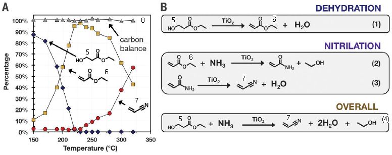
Start with Part B, on the right. This shows the new process, at two levels of detail. It's not important to follow all the detail, especially at the start, but we will use some of it as we go along.

The bottom section of Part B shows the overall process (equation 4). Compound 5 is converted to compound 7. Compound 7 is acrylonitrile, the desired product. Compound 5 is the ethyl ester of 3-hydroxypropanoic acid. Previous work had established a bacterial fermentation to make compound 5 from sugar; it is the starting material here.

The top two sections of Part B show the two steps -- one on each end of the starting compound. The first step is dehydration: removing the -OH group and an -H from the next C, leading to a double bond (equation 1). That gives compound 6, an intermediate here. The second step is to remove the ester group, and replace it with a nitrile group (equations 2-3). That gives compound 7, the desired product.

Part A shows an example of how this works. In this case, the overall process was run at various temperatures (T). The graph shows what happened as a function of T. For example, at the lowest T (150 °C), the process led to about 90% of the original compound 5, and 10% of the intermediate 6. There was essentially none of the desired product 7. That is, not much happened at this low T. With higher T, more and more 7 was obtained, reaching over 50% at the highest T shown here. The level of 6, the intermediate, first rises with T, then falls -- as more is converted to the final product.

The top line in the graph (labeled "8")? It's pretty much flat, at 100%. That's good; that's the sum of all the chemicals they analyzed. It's a test to see that the analyses make sense; all of the material is accounted for.

This is slightly modified from parts of Figure 1 in the article. I added more numbers for labeling. The authors numbered reactions 1-3 in part B. I added the numbers 4-8 for various equations, chemicals, and lines.

That's the idea, but the best yield is not very good. The authors went further, and did the two steps separately. The first step is done at a fairly low T, making the intermediate, compound 6. That product stream is passed on to a second reactor, at a higher T. Doing the two steps separately, at different T, leads to an overall yield of the desired product of about 98%. Excellent!

In addition to avoiding petroleum and having a high yield, the proposed process is actually simpler than the current process. And it avoids the release of hydrogen cyanide (HCN), so it may be safer, too. Nevertheless, we emphasize that the article is a presentation of something new, with only small-scale testing.

The article summarizes an economic projection for the process, suggesting that the product cost would be competitive with current prices, based on petroleum. These numbers are encouraging. However, the current price fluctuates, depending on market forces, and the projected prices have considerable uncertainty. Further, cost projections for new processes are usually optimistic. If nothing else, it takes a while to get a new process running efficiently.

News stories:
* A Sweet Approach to Renewable Acrylonitrile Production. (S Himmelstein, Engineering 360 (IEEE), December 8, 2017.) Includes a flow chart of the overall proposed process, as shown in Figure 3 of the article.
* NREL Develops Novel Method to Produce Renewable Acrylonitrile. (National Renewable Energy Laboratory (NREL), December 7, 2017.) From the lead institution.

The article: Renewable acrylonitrile production. (E M Karp et al, Science 358:1307, December 8, 2017.) Check Google Scholar for a freely available copy.

A post about acrylonitrile polymers: Fixing the heart with some glue and light (July 27, 2014). Acrylonitrile is called cyanoacrylate in this earlier post. As usual in organic chemistry, the prefix cyano and the suffix nitrile are interchangeable.

Another approach to making acrylates: Briefly noted... A pathway to renewable acrylate (March 18, 2023).

Another post proposing an improved way to make a chemical used in plastics: A simpler way to make styrene (July 10, 2015).

A post about use of titanium dioxide as a catalyst: Photocatalytic paints: do they, on balance, reduce air pollution? (September 17, 2017).

More TiO₂: How to "dye" carbon fiber -- with titanium dioxide (January 20, 2018).

A broad view of plastics... History of plastic -- by the numbers (October 23, 2017).

More plastics: Follow-up: bacterial degradation of PET plastic (April 25, 2018).

This post is listed on my page Internet Resources for Organic and Biochemistry in the section for Carboxylic acids, etc.

Treating obesity: A microneedle patch to induce local fat browning

January 5, 2018

This post ties together several issues that have come up before. They include...
- brown fat, especially the more specific issue of beige fat;
- the implications of developing beige fat for obesity, and also for diabetes;
- the use of microneedle patches to deliver a drug through the skin.

There are some background links about those issues at the end, but the key biology issue is the beige fat. Our traditional view of fat is that it is an energy reserve. We store fat for later use, when food is scarce. Of course, if we don't use it later, we get obese. We now recognize a second type of fat cell, which actively burns fat molecules -- without collecting the energy in any useful form, except heat. This "thermogenic" fat is called brown fat. (Its brown color is due to a high level of mitochondria, with their brown cytochromes.) Beige fat is a type of brown fat; more specifically it is brown fat made from the ordinary storage (or "white") fat. Since brown fat burns food without collecting the energy, it seems logical that it might be useful in preventing weight gain. Since the brown fat affects energy metabolism, perhaps it would have an impact on diabetes.

The stories of brown -- and especially beige -- fat are fairly new. We are beginning to understand them, but still have little idea how we might make use of the information.

A new article explores a way to exploit beige fat. The scientists have a drug that stimulates the conversion of ordinary white fat calls to beige fat cells. They deliver the drug, locally, through the skin by use of a microneedle patch. They then observe what happens.

The study is done with mice, with diet-induced obesity.

Here is the idea...

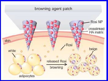
Start with the layer of skin. Below it are some fat cells (adipocytes). Above it is a microneedle patch, labeled "browning agent patch", with three of the needles penetrating the skin.

The patch contains a drug called rosiglitazone (Rosi), which is packaged in nanoparticles (NP) in the patch. The drug is slowly released under the skin. It then converts some of the white fat cells to beige fat cells.

This is the Figure from the abstract of the article.

Here is an example of the results...

This is a glucose tolerance test. A big dose of glucose is given; the blood sugar level is measured over time. You can see that it rises rapidly due to the glucose that was given. It then falls.

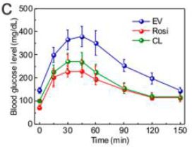
The two main curves here are "EV" (blue, top) and "Rosi" (red, bottom). Rosi is the drug; EV stands for empty vehicle -- a mock needle patch without any drug.

You can see that the mock EV treatment shows a high peak glucose level, but the Rosi treatment results in a lower peak.

There is a third curve, labeled "CL" (green). It is for a different drug. The results for the two drugs, Rosi and CL, are similar.

This is Figure 5c from the article.

The results show that the drugs improved glucose tolerance in this mouse model. Other data show that the drugs reduced weight gain. Overall, the article shows that induced browning of fat can be of practical benefit, and that the microneedle patch is an effective delivery tool. The patch allows local slow-but-sustained delivery; it may be a "gentle" way to provide the drug. Thus it may minimize some of the problems that have been observed with systemic delivery of such drugs.

We noted at the outset that our understanding of brown and beige fat is new and limited. That holds, too, for steps toward treatment. The current article is an interesting step, but it is important to understand how early it is.

News stories:
* Microneedle skin patch that delivers fat-shrinking drug locally could be used to treat obesity and diabetes. (Phys.org, September 15, 2017.)
* Nanoparticle Drug Delivery Patch for Obesity Treatment. (B Cuffari, AZoNano, September 21, 2017.)

The article: Locally Induced Adipose Tissue Browning by Microneedle Patch for Obesity Treatment. (Y Zhang et al, ACS Nano 11:9223, September 26, 2017.)

Background posts include ...
* Beige fat, with a connection to obesity: An obesity gene: control of brown fat (October 2, 2015).
* A post on diabetes, including glucose tolerance tests: Making a functional mouse pancreas in a rat (February 17, 2017).
* Microneedle patches: Clinical trial of self-administered patch for flu immunization (July 31, 2017).

More about obesity: Using a zipper to prevent obesity (September 25, 2018).

More microneedles: Treating a heart attack using a microneedle patch (January 11, 2019).

More drug delivery: Making a small container that has an opening in it (September 10, 2019).

For more about fats, see the section of my page Organic/Biochemistry Internet resources on Lipids. It includes a list of related Musings posts, including posts on obesity.

More on diabetes is on my page Biotechnology in the News (BITN) -- Other topics under Diabetes. That includes a list of related Musings posts.

January 3, 2018

Diagnosing diabetes in people of African ancestry: a race-dependent variable

January 3, 2018

Diabetes is a disorder that affects the level of glucose in the blood. Of course, blood sugar level varies. A single measurement of the level is just one snapshot.

One way to diagnose diabetes is to measure a stable change that accumulates over time depending on the blood sugar. A useful example is glycated hemoglobin, a product of the hemoglobin reacting with the sugar. A single measurement of glycated hemoglobin integrates the entire history of the person's blood glucose level over the lifetime of the red blood cells (RBC).

It is known that there are factors other than diabetes that can affect the level of glycated hemoglobin, but doctors still find the measurement useful. for both diagnosis and monitoring.

A recent article reports a special problem with the glycated hemoglobin measurement in people of African ancestry.

The following graph summarizes some of the key results. We'll work through it slowly; it takes a while to get to the important data.

The y-axis shows the amount of glycated hemoglobin found in the blood of various groups of people. All the people studied here were thought to be free of diabetes.

The x-axis is labeled by ancestry and GS. The GS is the genetic score, a measure of how many genetic variants the person has that seem to have some effect on the glycation level.

To get the idea of the graph, look at the first group of measurements, at the left. These are for people of European ancestry. The three points are for the lowest 5% of the distribution, the middle 90%, and the top 5%. The values for glycated hemoglobin range from about 5.2 to 5.6 for these points. This shows that genetic variation does affect the level of glycation.

The second group of three points is for a sub-population of those of European ancestry. The results are similar.

The next two groups of data are for people of Asian ancestry. For these people, the range of values is smaller.

And now, the "important" part... The next two data sets are for people of African ancestry. There is a now a very wide range of values. In particular, the scores for the lowest 5% of those of African ancestry are very low compared to the scores for the other groups.

This is Figure 5 from the article.

That is, some people of African ancestry have an unusually low level of glycated hemoglobin. This is shown on the graph by the average value for the lowest 5%. It is about 5.0 for Africans, over 5.2 for the other groups.

What is it due to? A particular mutation in the gene for the enzyme glucose-6-phosphate dehydrogenase (G6PD). This is a gene on the X chromosome, so men have only one copy. Look at the last (right-most) set of data on the graph above. It is for African-ancestry men ("AA men"). Those who have the base T at this site have a glycated hemoglobin level of about 5.0. Those who have C at that site have about 5.8.

Next to that data set are the results for AA women. They have two copies of the gene, of course, so the situation is a little more complicated. But the general pattern is the same. T leads to low glycation.

What does this mutation do? It affects the lifetime of the RBC. The allele with T leads to short-lived RBC. If the RBC don't live as long, they don't accumulate as much modified hemoglobin. That is, we understand how the T allele leads to low glycation.

The point is that the T allele could interfere with the diagnosis of diabetes, by leading to a low level of glycation that is not reflecting the actual blood sugar level. The authors note that this T allele is almost unique to people of African ancestry. About 11% of African Americans have a T; "almost no one of any other ancestry" [author summary, p7] has it. It thus seems clear that this is a race-related variable that could bias the detection of diabetes.

The current article does not provide specific information on how the newly discovered mutation affects glycation level in diabetics. That remains for future work, as does then working out what an appropriate response should be. For example, it might be appropriate to check for the G6PD mutation as part of diabetes screening, at least for those of African ancestry.

News story: Type 2 diabetes is being misdiagnosed in African-Americans, genetic study suggests. (EurekAlert!, September 12, 2017.)

The article, which is freely available: Impact of common genetic determinants of Hemoglobin A1c on type 2 diabetes risk and diagnosis in ancestrally diverse populations: A transethnic genome-wide meta-analysis. (E Wheeler et al, PLoS Medicine 14:e1002383, September 12, 2017.)

Other posts about race differences include...
* Alcohol consumption, an "ethnic" mutation, and a possible new drug (October 28, 2014).
* Why African-Americans have a high rate of kidney disease: another gene that is both good and bad (August 17, 2010).

Previous post on diabetes... Making a functional mouse pancreas in a rat (February 17, 2017).

Next, also about diagnosis... Diabetes: types 1, 2, 3, 4, 5 (March 16, 2018).

There is a section of my page Biotechnology in the News (BITN) -- Other topics on Diabetes. It includes a list of related Musings posts.

Another effect of some mutations in the G6PD gene: Genes that protect against malaria (January 19, 2010).

The spider with the mostest ... (and such)

January 2, 2018

Most mass... Specimens of this spider as heavy as 170 grams have been found.

It is Theraphosa blondi, the Goliath bird-eater.

170 grams is more than 1/3 of a pound. More than an ordinary hamburger patty.

This spider is also one of the "Most delicious." Roasted.

This is reduced from the first figure in the news story by Moscato. Figure 3A of the article shows a specimen of this spider, but the figure here is better for sense of scale.

And at the right...

Most web... As much as 2.8 square meters.

Made by a Caerostris darwini, Darwin's bark spider.

The creature at the bottom is presumably about 2 meters tall -- or at least was before the photographer truncated him. The spider? Don't know if it is visible in there. However, there is one featured in part e of the full figure in the article.

This is Figure 3f from the article.

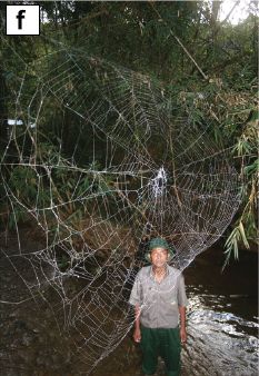
There are 96 more spider records in the article. Some are quantitative, some qualitative or subjective (such as "most delicious", mentioned above). Some are the biggest for some feature, some the smallest. Most are about the spiders themselves from nature. A few are about odd things from the lab (such as a ten-legged spider); a few are about those who study spiders.

Let's end this with a quiz... The spider Dipoena santaritadopassaquatrensis. What record does it hold? You may be able to guess from the information given here. You can check yourself in the article.

News story: Only the very best make it into the 'spider world records'. (D Moscato, Earth Touch News, November 6 2017.)

The article, which is freely available: Record breaking achievements by spiders and the scientists who study them. (S Mammola et al, PeerJ 5:e3972, October 31, 2017.) It's fun to browse. The authors' purpose is to promote interest in spiders. There are many pictures, though perhaps not enough.

The article says that the spider records will be maintained -- and updated -- as a web page at the site for the International Society of Arachnology. I don't see it there, so maybe it is just a plan for now. If anyone finds it, let me know.

* * * * *

Among spider posts in Musings...
* Provision of milk and maternal care in a spider (January 13, 2019).
* How a spider can help you do better microscopy (September 9, 2016).
* What to do if your brain won't fit in your head (February 18, 2012). The spider discussed in this post is noted under "largest central nervous system."
* How to seat a spider in front of the computer (September 28, 2010). The purpose here is to give the spider an eye exam. That's not easy with a spider, especially one that has eight eyes. The article notes various things about spider vision -- and hearing. Also, jumping spiders (a large group) are often mentioned.
* Spiders (December 21, 2009). Peacock spiders. The winner for "most elaborate courtship." This post also notes (with pictures) the happy-face spider. It's relative, the Caribbean smiley-faced spider, is the winner for "genus with most species named after celebrities."
* The vegetarian spider (October 21, 2009). The winner for "strangest diet."

The last time Musings started a new year with a post on arthropods... A new year (January 1, 2010).

Older items are on the page Musings: September-December 2017 (archive).

Top of page

The main page for current items is Musings.
The first archive page is Musings Archive.

E-mail announcement of the new posts each week -- information and sign-up: e-mail announcements.

Contact information Site home page

Last update: March 15, 2024